Validation and Benchmark of Wasserstein Distances • phutil

library(ggplot2)
library(phutil)

This vignette introduces the Wasserstein and bottleneck distances between persistence diagrams and their implementations in {phutil}, adapted from Hera, by way of two tasks:

Validate the implementations on an example computed by hand.
Benchmark the implementations against those provided by {TDA} (adapted from Dionysus).

We will also use the {tdaunif} package to generate larger point clouds and the {microbenchmark} package to perform benchmark tests.

Definitions

Persistence diagrams are multisets (sets with multiplicity) of points in the plane that encode the interval decompositions of persistent modules obtained from filtrations of data (e.g. Vietoris–Rips filtrations of point clouds and cubical filtrations of numerical arrays). Most applications consider only ordinary persistent homology, so that all points live in the upper-half plane; and most involve non-negative-valued filtrations, so that all points live in the first quadrant. The examples in this vignette will be no exceptions.

We’ll distinguish between persistence diagrams, which encode usually encode one degree of a persistence module, and persistence data, which comprises persistent pairs of many degrees (and annotated as such). Whereas a diagram is typically represented as a 2-column matrix with columns for birth and death values, data are typically represented as a 3-column matrix with an additional column for (whole number) degrees.

The most common distance metrics between persistence diagrams exploit the family of Minkowski distances $D_p$ between points in $\mathbb{R}^n$ defined, for $1 \leq p < \infty$ , as follows:

$D_p(x,y) = \left(\sum_{i=1}^{n}{(x_i - y_i)^p}\right)^{1/p}.$

In the limit $p \to \infty$ , this expression approaches the following auxiliary definition:

$D_\infty(x,y) = \max_{i=1}^{n}{\lvert x_i - y_i \rvert}.$

As the parameter $p$ ranges between $1$ and $\infty$ , three of its values yield familiar distance metrics: The taxicab distance $D_1$ , the Pythagorean distance $D_2$ , and the Chebyshev distance $D_\infty$ .

The Kantorovich or Wasserstein metric derives from the problem of optimal transport: What is the minimum cost of relocating one distribution to another? In the space of persistence diagrams, only finitely many points lie off the diagonal, though every point on the diagonal is taken to be included with multiplicity $\mathbb{N}$ . So the cost of relocating one diagram $X$ to another $Y$ amounts to (a) the cost of relocating some off-diagonal points to other off-diagonal points plus (b) the cost of relocating the remaining off-diagonal points to the diagonal (and vice-versa). This cost then depends entirely on how the off-diagonal points are matched, where a matching is any bijective map $\varphi : X \to Y$ , though in practice we assume that almost all diagonal points are matched to themselves and incur no cost.

The cost $D(x,\varphi(x))$ of relocating a point $x$ to its matched point $\varphi(x)$ is typically taken to be a Minkowski distance $D_q(x,\varphi(x)) = \lVert x - \varphi(x) \rVert_q$ , defined by the $L^q$ norm on $\mathbb{R}^2$ . (While simple, this geometric treatment elides that the points in the plane encode the collection of interval modules into which the persistence module decomposes. Other metrics have been proposed for this space, but we restrict to this family here.)

The total cost of the relocation is canonically taken to be the Minkowski distance $\left( \sum_{x \in X}{D(x,\varphi(x))^p} \right)^{1/p}$ of the vector of matched-point distances. The Wasserstein distance is defined to be the infimum of this value over all possible matches. This yields the formulae

$W_p^q(X,Y) = \inf_{\varphi : X \to Y}{\left( \sum_{x \in X}{{\lVert x-\varphi(x) \rVert_q}^p} \right)^{1/p}},$

for $p < \infty$ and

$W_\infty^q(X,Y) = \inf_{\varphi : X \to Y}{\max_{x \in X}{\lVert x-\varphi(x) \rVert_q}}$

for $p = \infty$ .

See Cohen-Steiner et al. (2010) and Bubenik, Scott, and Stanley (2023) for detailed treatments and stability results on these families of metrics.

Validation

Distances between nontrivial diagrams

The following persistence diagrams provide a tractable example:

$X = \left[ \begin{array}{cc} 1 & 3 \\ 3 & 5 \end{array} \right], \phantom{X = Y} Y = \left[ \begin{array}{cc} 3 & 4 \end{array} \right].$

For convenience in the code, we omit dimensionality and focus only on the matrix representations.

X <- rbind(
  c(1, 3),
  c(3, 5)
)
Y <- rbind(
  c(3, 4)
)

We overlay both diagrams in Figure 1. Note that the vector between the off-diagonal points $(1,3)$ of $X$ and $(3,4)$ of $Y$ is $(2,1)$ , while the vector from $(1,3)$ to its nearest diagonal point $(2,2)$ is $(1,-1)$ . That one coordinate is the same size while the other is smaller implies that an optimal matching will always match $(1,3)$ with the diagonal, so long as $p \geq 1$ . A similar argument necessitates that $(3,4)$ of $Y$ must match with $(3,5)$ of $X$ .

par(mar = c(4, 4, 1, 1) + .1)
plot(
  NA_real_,
  xlim = c(0, 6), ylim = c(0, 6), asp = 1, xlab = "birth", ylab = "death"
)
abline(a = 0, b = 1)
points(X, pch = 1)
points(Y, pch = 5)
segments(X[, 1], X[, 2], c(2, Y[, 1]), c(2, Y[, 2]), lty = 2)
par(mar = c(5, 4, 4, 2) + .1)

Figure 1: Overlaid persistence diagrams $X$ (circles) and $Y$ (diamond) with dashed segments connecting optimally matched pairs.

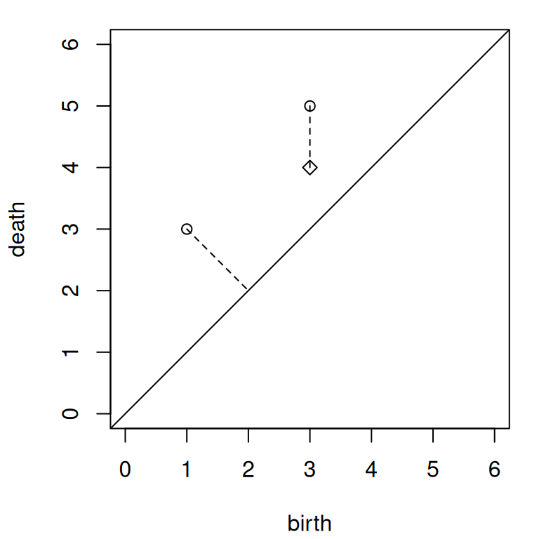
Based on these observations, we get this expression for the Wasserstein distance using the $q$ -norm half-plane metric and the $p$ -norm “matched space” metric:

$W_p^q(X,Y) = ( {\lVert a \rVert_q}^p + {\lVert b \rVert_q}^p )^{1/p},$

where $a = (1,-1)$ and $b = (0,-1)$ are the vectors between matched points. We can now calculate Wasserstein distances “by hand”; we’ll consider those using the half-plane Minkowski metrics with $q=1,2,\infty$ and the “matched space” metrics with $p=1,2,\infty$ .

First, with $q=1$ , we get $\lVert a \rVert_q = 1+1=2$ and $\lVert b \rVert_q = 0+1=1$ . So the $(1,p)$ -Wasserstein distance will be the $p$ -Minkowski norm of the vector $(2,1)$ , given by $W_p^1(X,Y) = (2^p + 1^p)^{1/p}$ . This nets us the values $W_1^1(X,Y) = 3$ and $W_2^1(X,Y) = \sqrt{5}$ . And then $W_\infty^1(X,Y) = \max(2,1) = 2$ . The reader is invited to complete the rest of Table 1.

Table 1: Distances between optimally paired features and Wasserstein distances between

X

and

Y

for several choices of half-plane and “matched space” metrics.

Metric	$\lVert a \rVert$	$\lVert b \rVert$	$W_1$	$W_2$	$W_\infty$
$L^1$	2	1	3	$\sqrt{5}$	2
$L^2$	$\sqrt{2}$	1	$1+\sqrt{2}$	$\sqrt{3}$	$\sqrt{2}$
$L^\infty$	1	1	2	$\sqrt{2}$	1

The results make intuitive sense; for example, the values change monotonically along each row and column. Let us now validate the bottom row—using the $L^\infty$ distance on the half-plane, giving the popular bottleneck distance—using both Hela, as exposed through {phutil}, and Dionysus, as exposed through {TDA}:

wasserstein_distance(X, Y, p = 1)
#> [1] 2
wasserstein_distance(X, Y, p = 2)
#> [1] 1.414214
bottleneck_distance(X, Y)
#> [1] 1

In order to compute distances with {TDA}, we must restructure the PDs to include a "dimension" column. Note also that TDA::wasserstein() does not take the $1/p$ th power after computing the sum of $p$ th powers; we do this manually to get comparable results:

TDA::wasserstein(cbind(0, X), cbind(0, Y), p = 1, dimension = 0)
#> [1] 2
sqrt(TDA::wasserstein(cbind(0, X), cbind(0, Y), p = 2, dimension = 0))
#> [1] 1.414214
TDA::bottleneck(cbind(0, X), cbind(0, Y), dimension = 0)
#> [1] 1

Distances from the trivial diagram

An important edge case is when one persistence diagram is trivial, i.e. contains only the diagonal so is “empty” of off-diagonal points. This can occur unexpectedly in comparisons of persistence data, as the data may be large but higher-degree features present in one set but absent in another. To validate the distances in this case, we create an empty diagram $E$ and use the same code to compare it to $X$ . The point $(3,5)$ of $X$ will be matched to the diagonal $(4,4)$ , which yields the same $\infty$ -distance $1$ so the $L^\infty$ Wasserstein distances will be the same as before.

# empty PD
E <- matrix(NA_real_, nrow = 0, ncol = 2)
# with dimension column
E_ <- cbind(matrix(NA_real_, nrow = 0, ncol = 1), E)
# distance from empty using phutil/Hera
wasserstein_distance(E, X, p = 1)
#> [1] 2
wasserstein_distance(E, X, p = 2)
#> [1] 1.414214
bottleneck_distance(E, X)
#> [1] 1
# distance from empty using TDA/Dionysus
TDA::wasserstein(E_, cbind(0, X), p = 1, dimension = 0)
#> [1] 2
sqrt(TDA::wasserstein(E_, cbind(0, X), p = 2, dimension = 0))
#> [1] 1.414214
TDA::bottleneck(E_, cbind(0, X), dimension = 0)
#> [1] 1

Benchmarks

For a straightforward benchmark test, we compute PDs from point clouds sampled with noise from two one-dimensional manifolds embedded in $\mathbb{R}^3$ : the circle as a trefoil knot and the segment as a two-armed archimedian spiral. To prevent the results from being sensitive to an accident of a single sample, we generate lists of 24 samples and benchmark only one iteration of each function on each.

set.seed(28415)
n <- 24
PDs1 <- lapply(seq(n), function(i) {
  S1 <- tdaunif::sample_trefoil(n = 120, sd = .05)
  as_persistence(TDA::ripsDiag(S1, maxdimension = 2, maxscale = 6))
})
PDs2 <- lapply(seq(n), function(i) {
  S2 <- cbind(tdaunif::sample_arch_spiral(n = 120, arms = 2), 0)
  S2 <- tdaunif::add_noise(S2, sd = .05)
  as_persistence(TDA::ripsDiag(S2, maxdimension = 2, maxscale = 6))
})

Both implementations are used to compute distances between successive pairs of diagrams. The computations are annotated by homological degree and Wasserstein power so that these results can be compared separately.

PDs1_ <- lapply(lapply(PDs1, as.data.frame), as.matrix)
PDs2_ <- lapply(lapply(PDs2, as.data.frame), as.matrix)
# iterate over homological degrees and Wasserstein powers
bm_all <- list()
PDs_i <- seq_along(PDs1)
for (dimension in seq(0, 2)) {
  # compute
  bm_1 <- do.call(rbind, lapply(seq_along(PDs1), function(i) {
    as.data.frame(microbenchmark::microbenchmark(
      TDA = TDA::wasserstein(
        PDs1_[[i]], PDs2_[[i]], dimension = dimension, p = 1
      ),
      phutil = wasserstein_distance(
        PDs1[[i]],  PDs2[[i]],  dimension = dimension, p = 1
      ),
      times = 1, unit = "ns"
    ))
  }))
  bm_2 <- do.call(rbind, lapply(seq_along(PDs1), function(i) {
    as.data.frame(microbenchmark::microbenchmark(
      TDA = sqrt(TDA::wasserstein(
        PDs1_[[i]], PDs2_[[i]], dimension = dimension, p = 2
      )),
      phutil = wasserstein_distance(
        PDs1[[i]],  PDs2[[i]],  dimension = dimension, p = 2
      ),
      times = 1, unit = "ns"
    ))
  }))
  bm_inf <- do.call(rbind, lapply(seq_along(PDs1), function(i) {
    as.data.frame(microbenchmark::microbenchmark(
      TDA = TDA::bottleneck(
        PDs1_[[i]], PDs2_[[i]], dimension = dimension
      ),
      phutil = bottleneck_distance(
        PDs1[[i]],  PDs2[[i]],  dimension = dimension
      ),
      times = 1, unit = "ns"
    ))
  }))
  # annotate and combine
  bm_1$power <- 1; bm_2$power <- 2; bm_inf$power <- Inf
  bm_res <- rbind(bm_1, bm_2, bm_inf)
  bm_res$degree <- dimension
  bm_all <- c(bm_all, list(bm_res))
}
bm_all <- do.call(rbind, bm_all)

Figure 2 compares the distributions of runtimes by homological degree (column) and Wasserstein power (row). We use nanoseconds in {microbenchmark} when benchmarking to avoid potential integer overflows. Hence, we convert the results into seconds ahead of formatting the axis in seconds.

bm_all <- transform(bm_all, expr = as.character(expr), time = unlist(time))
bm_all <- subset(bm_all, select = c(expr, degree, power, time))
ggplot(bm_all, aes(x = time * 10e-9, y = expr)) +
  facet_grid(
    rows = vars(power), cols = vars(degree),
    labeller = label_both
  ) +
  geom_violin() +
  scale_x_continuous(
    transform = "log10",
    labels = scales::label_timespan(units = "secs")
  ) +
  labs(x = NULL, y = NULL)

Figure 2: Benchmark comparison of Dionysus via {TDA} and Hera via {phutil} on large persistence diagrams: Violin plots of runtime distributions on a common scale.

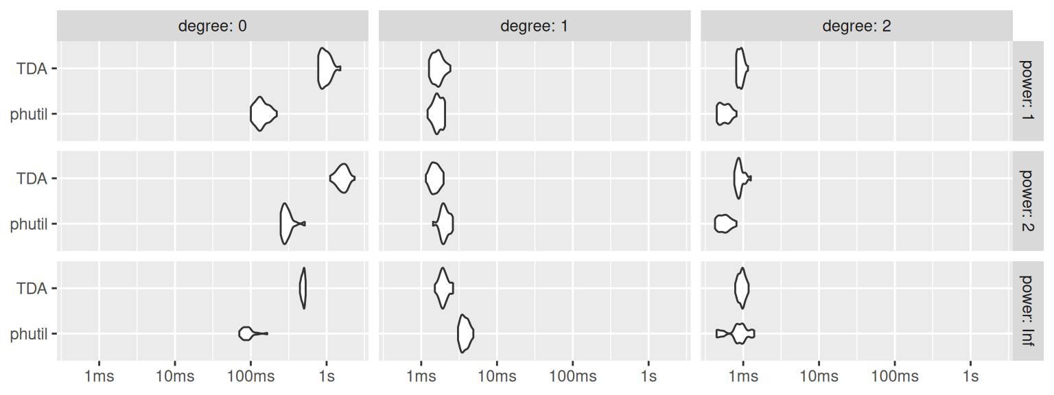
We note that Dionysus via {TDA} clearly outperforms Hera via {phutil} on degree-1 PDs, which in these cases have many fewer features. However, the tables are turned in degree 0, in which the PDs have many more features. (The implementations are more evenly matched on the degree-2 PDs, which may have to do with many of them being empty.) While by no means exhaustive and not necessarily representative, these results suggest that Hera via {phutil} scales more efficiently than Dionysus via {TDA} and should therefore be preferred for projects involving more feature-rich data sets.

References

Bubenik, Peter, Jonathan Scott, and Donald Stanley. 2023. “Exact Weights, Path Metrics, and Algebraic Wasserstein Distances.” Journal of Applied and Computational Topology 7 (2): 185–219.

Cohen-Steiner, David, Herbert Edelsbrunner, John Harer, and Yuriy Mileyko. 2010. “Lipschitz Functions Have l p-Stable Persistence.” Foundations of Computational Mathematics 10 (2): 127–39.