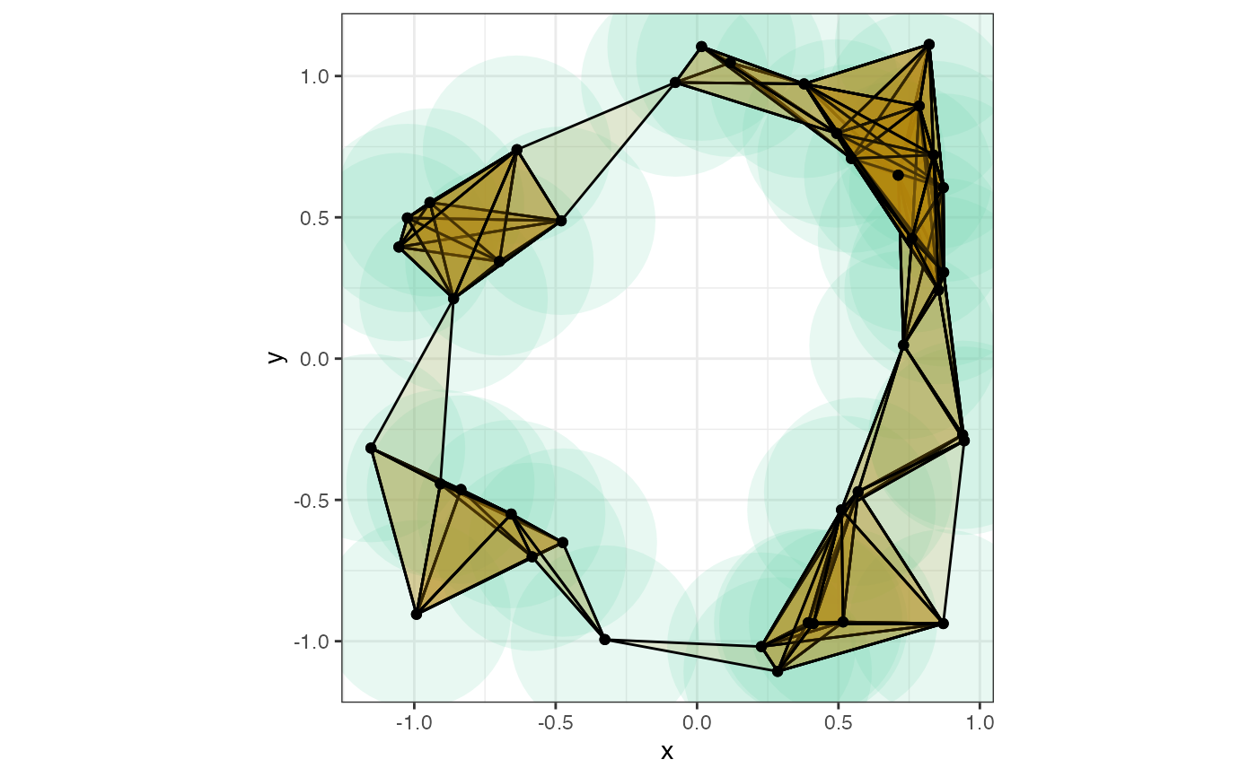
Simplicial complexes from 2-D point clouds

Construct and plot simplicial complexes that equal or approximate the topology of a ball cover of a set of points.

stat_simplicial_complex(
  mapping = NULL,
  data = NULL,
  geom = "SimplicialComplex",
  position = "identity",
  complex = "Rips",
  diameter = NULL,
  radius = NULL,
  dimension_max = 2L,
  zero_simplices = "all",
  one_simplices = "maximal",
  engine = NULL,
  na.rm = FALSE,
  show.legend = NA,
  inherit.aes = TRUE,
  ...
)

geom_simplicial_complex(
  mapping = NULL,
  data = NULL,
  stat = "SimplicialComplex",
  position = "identity",
  outlines = TRUE,
  na.rm = FALSE,
  show.legend = NA,
  inherit.aes = TRUE,
  ...
)

Arguments

mapping

Set of aesthetic mappings created by aes(). If specified and inherit.aes = TRUE (the default), it is combined with the default mapping at the top level of the plot. You must supply mapping if there is no plot mapping.

data

The data to be displayed in this layer. There are three options:

If NULL, the default, the data is inherited from the plot data as specified in the call to ggplot().

A data.frame, or other object, will override the plot data. All objects will be fortified to produce a data frame. See fortify() for which variables will be created.

A function will be called with a single argument, the plot data. The return value must be a data.frame, and will be used as the layer data. A function can be created from a formula (e.g. ~ head(.x, 10)).

geom

The geometric object to use to display the data, either as a ggproto Geom subclass or as a string naming the geom stripped of the geom_ prefix (e.g. "point" rather than "geom_point")

position

Position adjustment, either as a string naming the adjustment (e.g. "jitter" to use position_jitter), or the result of a call to a position adjustment function. Use the latter if you need to change the settings of the adjustment.

complex

The type of complex to compute, one of "Vietoris", "Rips" (equivalent), "Cech", or "alpha".

radius, diameter

The (positive) radius or diameter used in the construction. Provide only one of these; if neither is provided, they default to zero.

dimension_max

Compute simplices of dimension up to dimension_max (only relevant for the Vietoris--Rips complex computed with the simplextree engine).

zero_simplices

Which 0-simplices (vertices) to plot; one of "none", "maximal", and "all" (default).

one_simplices

Which 1-simplices (edges) to plot; one of "none", "maximal" (default), and "all".

engine

The computational engine to use (see 'Details'). Reasonable defaults are chosen based on complex.

na.rm

If FALSE, the default, missing values are removed with a warning. If TRUE, missing values are silently removed.

show.legend

logical. Should this layer be included in the legends? NA, the default, includes if any aesthetics are mapped. FALSE never includes, and TRUE always includes. It can also be a named logical vector to finely select the aesthetics to display.

inherit.aes

If FALSE, overrides the default aesthetics, rather than combining with them. This is most useful for helper functions that define both data and aesthetics and shouldn't inherit behaviour from the default plot specification, e.g. borders().

...

Other arguments passed on to layer(). These are often aesthetics, used to set an aesthetic to a fixed value, like colour = "red" or size = 3. They may also be parameters to the paired geom/stat.

stat

The statistical transformation to use on the data for this layer, either as a ggproto Geom subclass or as a string naming the stat stripped of the stat_ prefix (e.g. "count" rather than "stat_count")

outlines

Should the outlines of polygons representing high-dimensional simplices be drawn?

Details

Persistent homology is ultimately based on the topological properties of regions containing a set of points. When the region is the union of balls of a common radius, its homology is equal to or approximated by that of several families of simplicial complexes constructed on the point set. The simplicial complex stat constructs these simplicial complexes for a set of points in \(xy\)-space while the geom plots them on the same coordinates as the points.

Complexes

A Vietoris--Rips complex of a point cloud is the simplicial complex consisting of a simplex for each subset of points within a fixed diameter of each other. A Čech complex contains the simplex for each subset that lies within a circle of fixed diameter. (This means that the Čech complex depends on the geometry of the ambient space containing the point cloud, while the Vietoris complex depends only on the inter-point distances. Moreover, a Vietoris complex contains the Čech complex of the same diameter.) An alpha complex comprises those simplices of the Delaunay triangulation within a fixed diameter.

ggtda relies on four engines to compute simplicial complexes, which can be specified to the engine parameter: Vietoris--Rips and Čech complexes of dimension at most 2 are implemented in base R ("base"), which is slow but allows the package to stand alone for small cases. RTriangle::triangulate() is used to compute the Delaunay triangulation for alpha complexes ("RTriangle"), without inserting Steiner points (so that the vertices of the triangulation are among those of the data). The package TDA can compute Vietoris--Rips filtrations and alpha filtrations ("TDA" for default engines, or specify the "GUDHI" or "Dionysus" engine). Finally, the highly optimized package simplextree can be called to compute Vietoris--Rips complexes ("simplextree"). As other complexes are implemented in simplextree, they will be made available here.

Aesthetics

stat_simplicial_complex() understands the following aesthetics (required aesthetics are in bold):

x
y
group

geom_simplicial_complex() understands the following aesthetics (required aesthetics are in bold):

x
y
id
dimension
alpha
colour
fill
group
linetype
linewidth
shape
size
stroke

Learn more about setting these aesthetics in vignette("ggplot2-specs", package = "ggplot2").

Computed variables

stat_simplicial_complex calculates the following variables that can be accessed with delayed evaluation.

after_stat(dimension)
integer dimension of the corresponding simplex.
after_stat(id)
character simplex identifier within each dimension.
after_stat(face)
factor encoding of dimension for >= 2L-dimensional simplices.

Examples


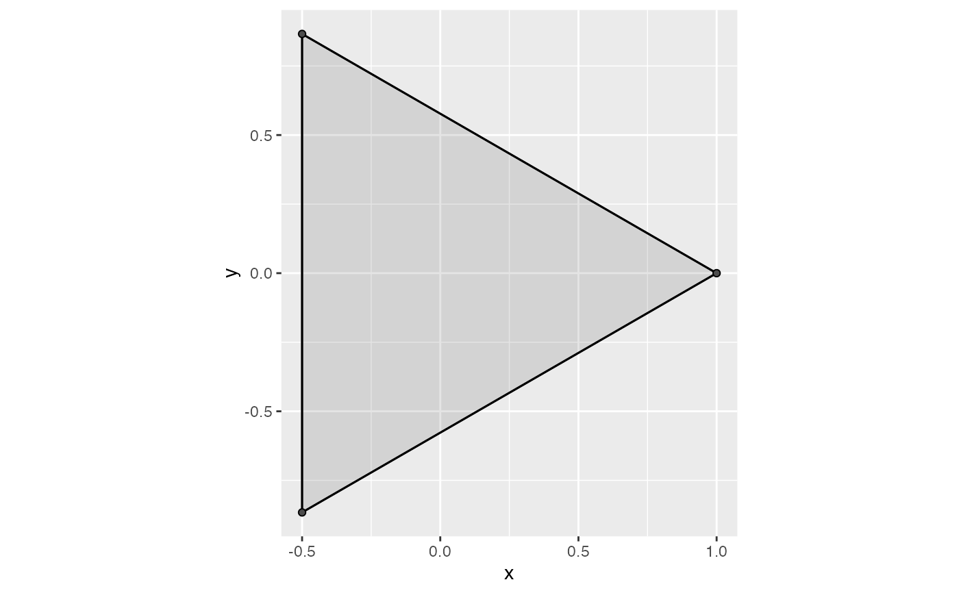
# equilateral triangle
equilateral_triangle <- 
  data.frame(x = cos(2*pi*c(0,1/3,2/3)), y = sin(2*pi*c(0,1/3,2/3)))
# small perturbations from key values
eps <- .00000001

# Vietoris-Rips
ggplot(equilateral_triangle, aes(x, y)) +
  coord_fixed() +
  geom_simplicial_complex(diameter = sqrt(3) - eps)

ggplot(equilateral_triangle, aes(x, y)) +
  coord_fixed() +
  geom_simplicial_complex(diameter = sqrt(3) + eps)


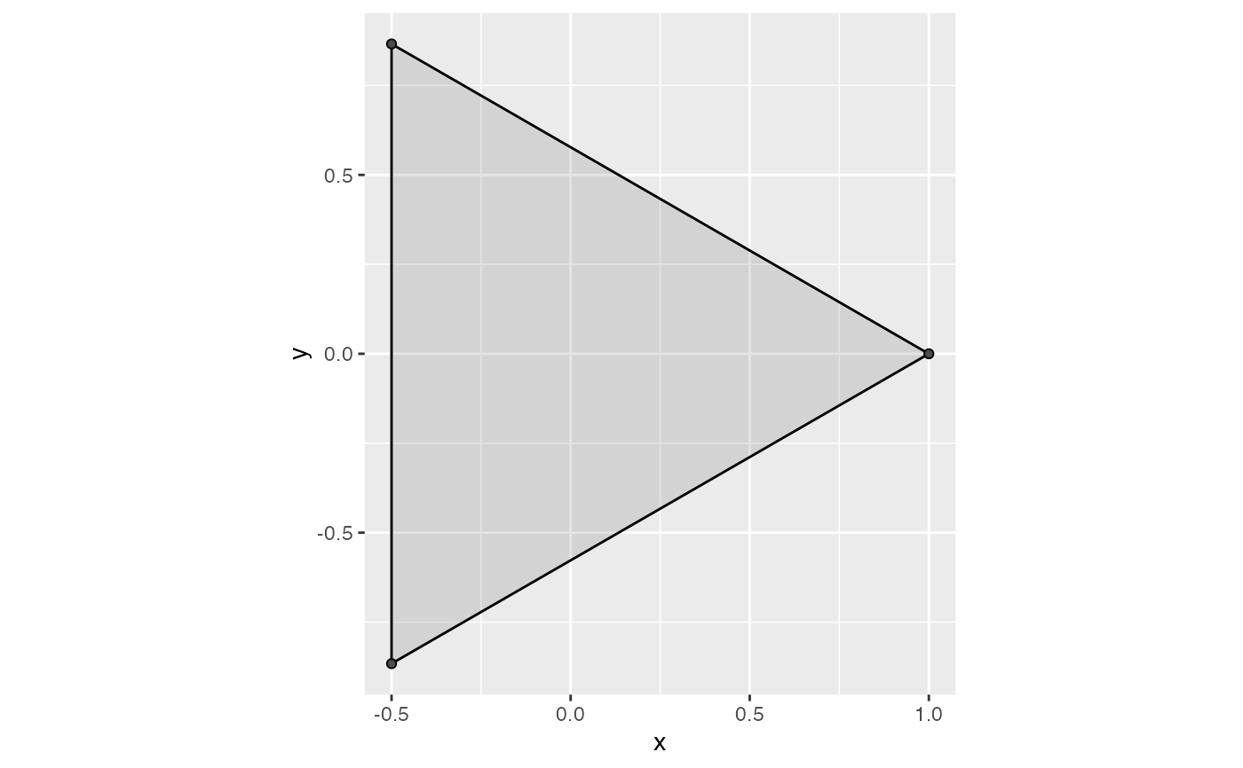# Čech
ggplot(equilateral_triangle, aes(x, y)) +
  coord_fixed() +
  geom_simplicial_complex(complex = "Cech", diameter = sqrt(3) - eps)

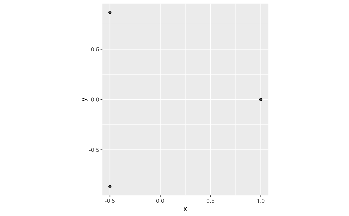ggplot(equilateral_triangle, aes(x, y)) +
  coord_fixed() +
  geom_simplicial_complex(complex = "Cech", diameter = sqrt(3) + eps)


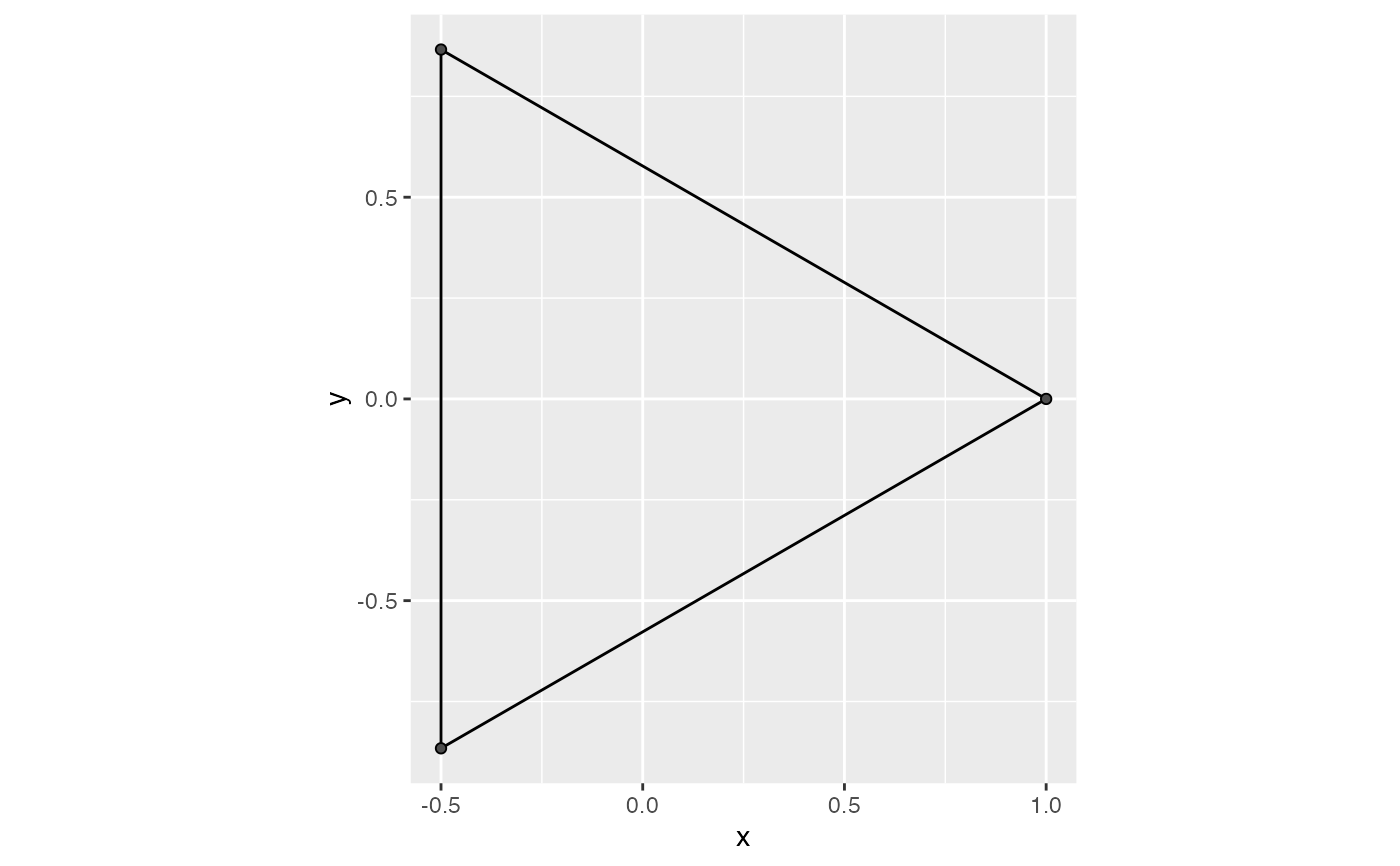# alpha
ggplot(equilateral_triangle, aes(x, y)) +
  coord_fixed() +
  geom_simplicial_complex(complex = "alpha", diameter = sqrt(3) - eps)

ggplot(equilateral_triangle, aes(x, y)) +
  coord_fixed() +
  geom_simplicial_complex(complex = "alpha", diameter = sqrt(3) + eps)


set.seed(1)
s <- seq(0, 2*pi, length.out = 40)
df <- data.frame(
  x = cos(s) + rnorm(40, 0, .1),
  y = sin(s) + rnorm(40, 0, .1)
)

# default
ggplot(df, aes(x, y)) +
  coord_fixed() +
  geom_simplicial_complex(radius = .4)

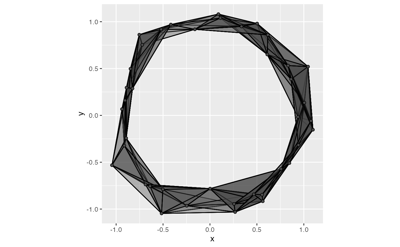
# higher-dimensional simplices are not more opaque but cause overlap
ggplot(df, aes(x, y)) +
  coord_fixed() +
  geom_simplicial_complex(radius = .4, dimension_max = 3L)


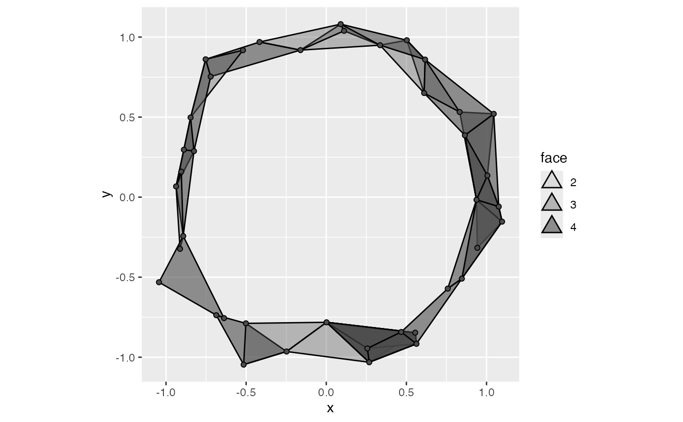
# visualizing dimension w/ face & alpha:
ggplot(df, aes(x, y)) +
  coord_fixed() +
  geom_simplicial_complex(
    mapping = aes(alpha = after_stat(face)),
    radius = .3, dimension_max = 4L
  ) +
  scale_alpha_ordinal(range = c(.1, .6))

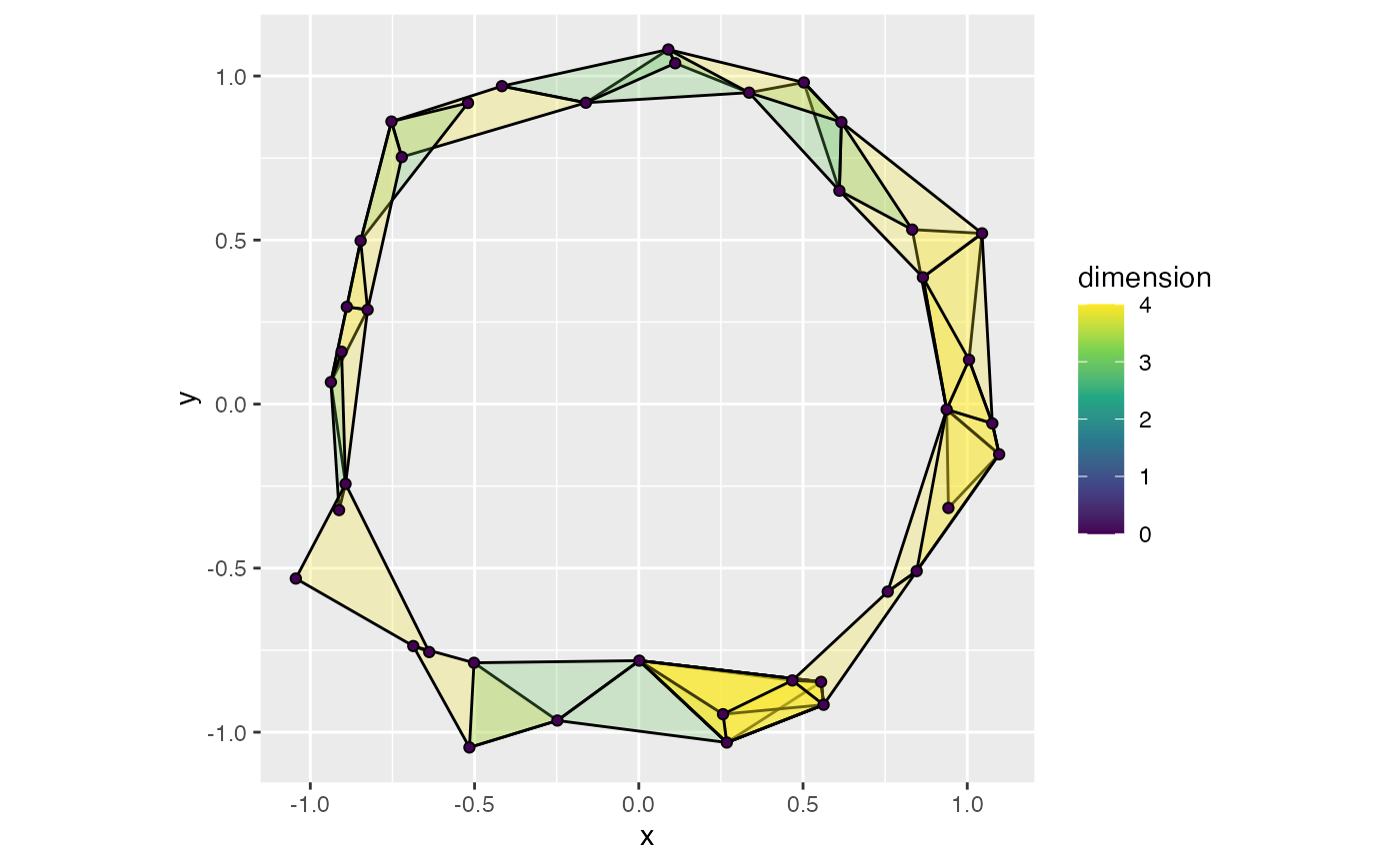
# visualizing dimension w/ dimension & fill:
ggplot(df, aes(x, y)) +
  coord_fixed() +
  geom_simplicial_complex(
    mapping = aes(fill = after_stat(dimension)),
    radius = .3, dimension_max = 4L, alpha = .25
  ) +
  scale_fill_continuous(type = "viridis")


# with a zero radius or diameter
ggplot(df, aes(x = x, y = y)) +
  coord_fixed() +
  stat_simplicial_complex(radius = 0)

# with a too-small radius or diameter
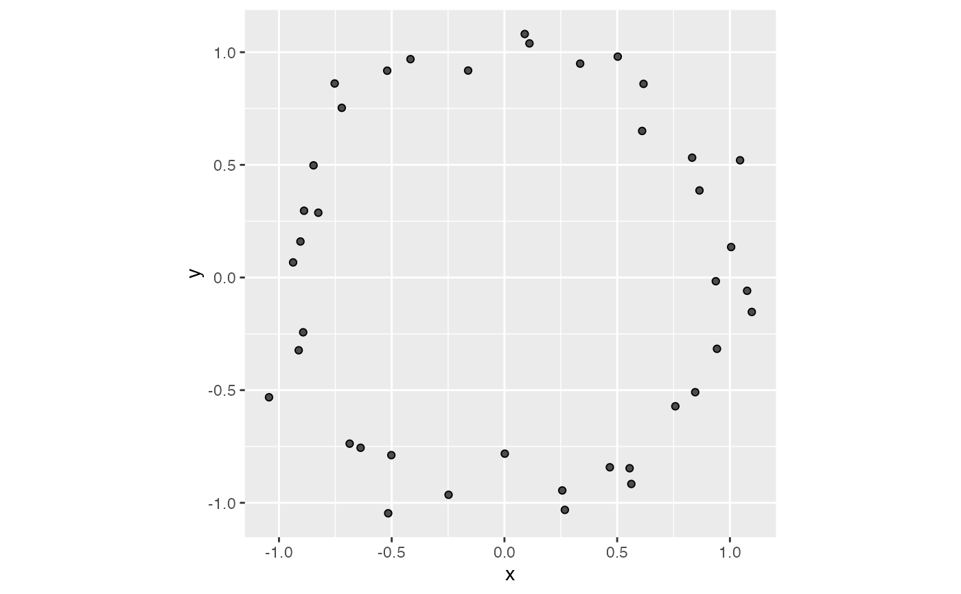
ggplot(df, aes(x = x, y = y)) +
  coord_fixed() +
  stat_simplicial_complex(radius = 0.01)


# Visualizing multiple groups together
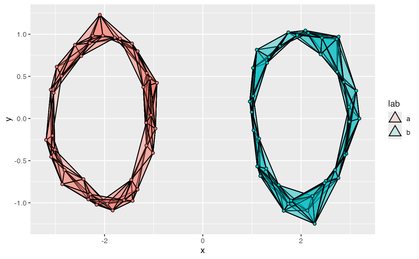
s <- c(s, s)
df_mix <- data.frame(
  x = cos(s) + rnorm(80, 0, .1),
  y = sin(s) + rnorm(80, 0, .1)
)
df_mix$x <- df_mix$x + rep(c(-2, 2), length.out = 80)
df_mix$lab <- rep(c("a", "b"), length.out = 80)

ggplot(df_mix, aes(x, y, fill = lab)) +
  geom_simplicial_complex(radius = .4)


# generate a noisy 2D circle
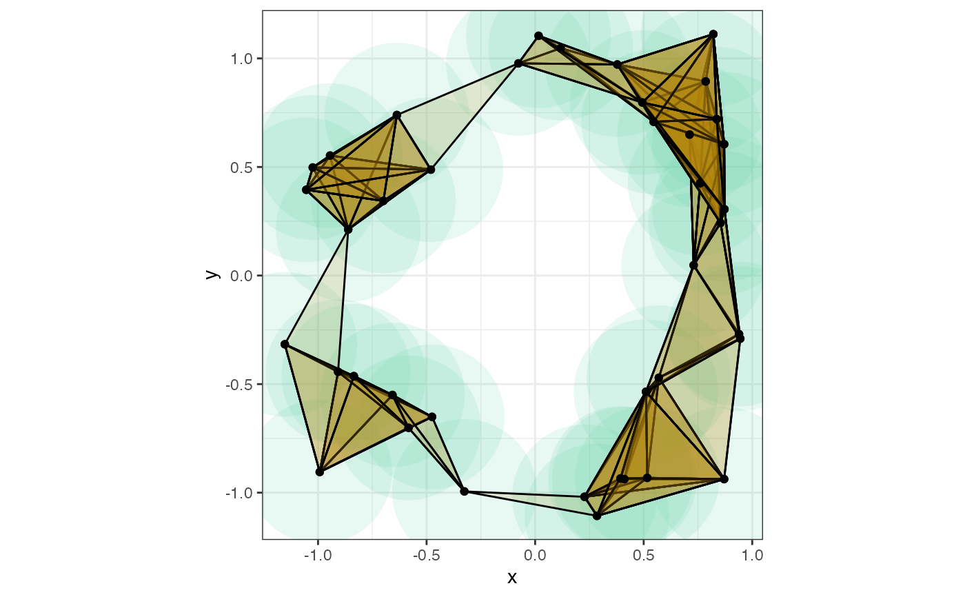
set.seed(2)
theta <- stats::runif(n = 40L, min = 0, max = 2*pi)
d <- data.frame(x = cos(theta) + stats::rnorm(40L, 0, .15),
                y = sin(theta) + stats::rnorm(40L, 0, .15))
r <- 1/3

# overlay ball cover and Vietoris-Rips complex with points
ggplot(d, aes(x = x, y = y)) +
  theme_bw() +
  coord_fixed() +
  geom_disk(radius = r, fill = "aquamarine3") +
  geom_simplicial_complex(
    radius = r, fill = "darkgoldenrod",
    complex = "Vietoris", engine = "base"
  ) +
  geom_point()

# use the Čech complex instead
ggplot(d, aes(x = x, y = y)) +
  theme_bw() +
  coord_fixed() +
  geom_disk(radius = r, fill = "aquamarine3") +
  geom_simplicial_complex(
    radius = r, fill = "darkgoldenrod",
    complex = "Cech", engine = "base"
  ) +
  geom_point()