Disk covers of 2-D point clouds

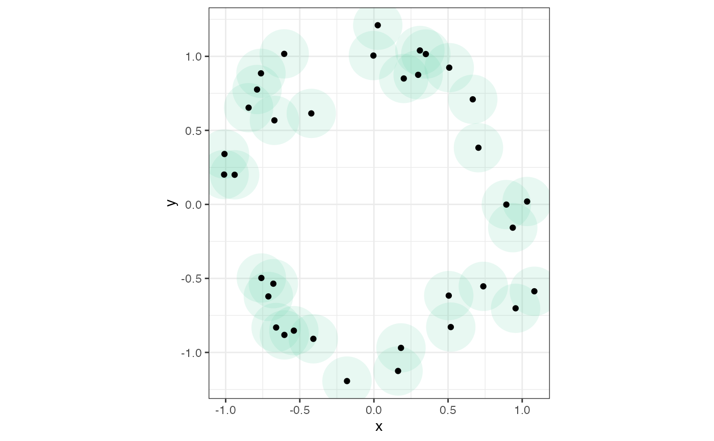
Center disks at points in a scatterplot.

geom_disk(
  mapping = NULL,
  data = NULL,
  stat = "identity",
  position = "identity",
  na.rm = FALSE,
  radius = NULL,
  diameter = NULL,
  segments = 60L,
  show.legend = NA,
  inherit.aes = TRUE,
  ...
)

Arguments

mapping

Set of aesthetic mappings created by aes(). If specified and inherit.aes = TRUE (the default), it is combined with the default mapping at the top level of the plot. You must supply mapping if there is no plot mapping.

data

The data to be displayed in this layer. There are three options:

If NULL, the default, the data is inherited from the plot data as specified in the call to ggplot().

A data.frame, or other object, will override the plot data. All objects will be fortified to produce a data frame. See fortify() for which variables will be created.

A function will be called with a single argument, the plot data. The return value must be a data.frame, and will be used as the layer data. A function can be created from a formula (e.g. ~ head(.x, 10)).

stat

The statistical transformation to use on the data for this layer, either as a ggproto Geom subclass or as a string naming the stat stripped of the stat_ prefix (e.g. "count" rather than "stat_count")

position

Position adjustment, either as a string naming the adjustment (e.g. "jitter" to use position_jitter), or the result of a call to a position adjustment function. Use the latter if you need to change the settings of the adjustment.

na.rm

Logical; ignored.

radius, diameter

The (positive) radius or diameter used in the construction. Provide only one of these; if neither is provided, they default to zero.

segments

The number of segments in the regular polygon that approximates each disk

show.legend

logical. Should this layer be included in the legends? NA, the default, includes if any aesthetics are mapped. FALSE never includes, and TRUE always includes. It can also be a named logical vector to finely select the aesthetics to display.

inherit.aes

If FALSE, overrides the default aesthetics, rather than combining with them. This is most useful for helper functions that define both data and aesthetics and shouldn't inherit behaviour from the default plot specification, e.g. borders().

...

Additional arguments passed to ggplot2::layer().

Details

A ball of radius \(r\) around a point \(x\) in Euclidean space consists of all points whose distances from \(x\) are less than \(r\). A ball in 2 dimensions is called a disk.

The geometric objects of GeomDisk can be used to illustrate disk covers of point clouds, in particular in the construction of simplicial filtrations. It could be paired with a statistical transformation of Stat* that samples points from a cloud.

The convenience function geom_disk() produces a layer with the identity statistical transformation.

Aesthetics

geom_disk() understands the following aesthetics (required aesthetics are in bold):

x
y
alpha
colour
fill
group
linetype
linewidth

Learn more about setting these aesthetics in vignette("ggplot2-specs", package = "ggplot2").

Examples


# function to generate noisy 2D circles
make_noisy_circle <- function(n, sd = .01) {
  theta <- stats::runif(n = n, min = 0, max = 2*pi)
  cbind(x = cos(theta) + stats::rnorm(n, 0, sd),
        y = sin(theta) + stats::rnorm(n, 0, sd))
}

# generate a noisy 2D circle
set.seed(1)
d <- as.data.frame(make_noisy_circle(n = 36L, sd = .15))
r <- 1/6

# plot disks beneath points
ggplot(d, aes(x = x, y = y)) +
  theme_bw() +
  coord_fixed() +
  geom_disk(radius = r, fill = "aquamarine3") +
  geom_point()

# use `diameter` parameter
ggplot(d, aes(x = x, y = y)) +
  theme_bw() +
  coord_fixed() +
  geom_disk(diameter = 2*r, fill = "aquamarine3") +
  geom_point()


# generate a noisy 2D circle
set.seed(2)
theta <- stats::runif(n = 40L, min = 0, max = 2*pi)
d <- data.frame(x = cos(theta) + stats::rnorm(40L, 0, .15),
                y = sin(theta) + stats::rnorm(40L, 0, .15))
r <- 1/3

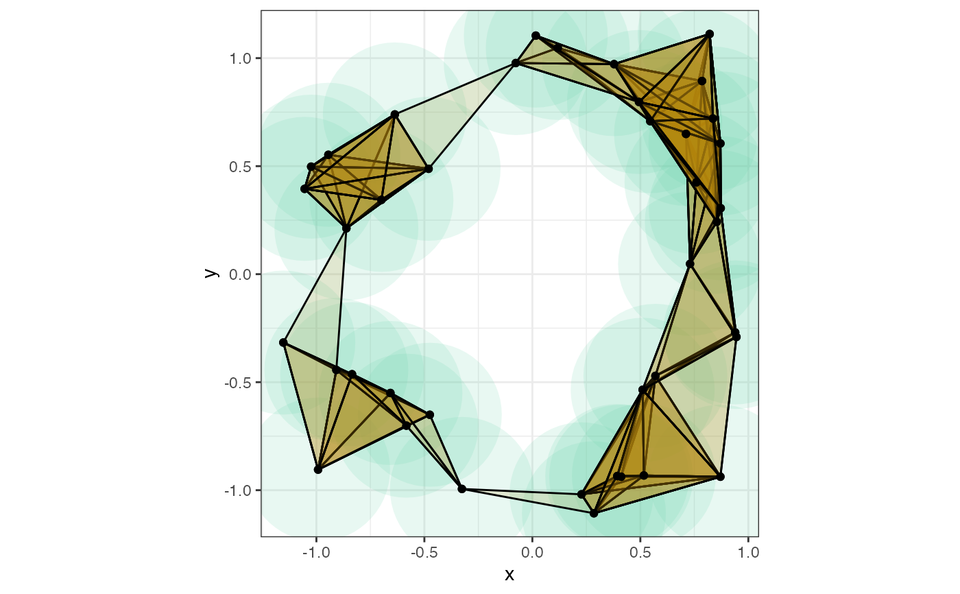
# overlay ball cover and Vietoris-Rips complex with points
ggplot(d, aes(x = x, y = y)) +
  theme_bw() +
  coord_fixed() +
  geom_disk(radius = r, fill = "aquamarine3") +
  geom_simplicial_complex(
    radius = r, fill = "darkgoldenrod",
    complex = "Vietoris", engine = "base"
  ) +
  geom_point()

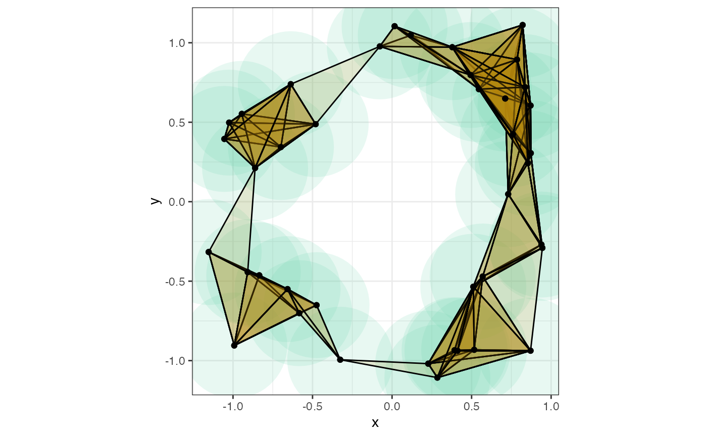
# use the Čech complex instead
ggplot(d, aes(x = x, y = y)) +
  theme_bw() +
  coord_fixed() +
  geom_disk(radius = r, fill = "aquamarine3") +
  geom_simplicial_complex(
    radius = r, fill = "darkgoldenrod",
    complex = "Cech", engine = "base"
  ) +
  geom_point()

Disk covers of 2-D point clouds

Arguments

Details

Aesthetics

See also

Examples