Persistence diagrams

Visualize persistence data in a (flat, diagonal, or landscape) persistence diagram.

stat_persistence(
  mapping = NULL,
  data = NULL,
  geom = "point",
  position = "identity",
  filtration = "Rips",
  diameter_max = NULL,
  radius_max = NULL,
  dimension_max = 1L,
  field_order = 2L,
  engine = NULL,
  order_by = c("persistence", "start"),
  decreasing = FALSE,
  diagram = "diagonal",
  na.rm = FALSE,
  show.legend = NA,
  inherit.aes = TRUE,
  ...
)

geom_fundamental_box(
  mapping = NULL,
  data = NULL,
  stat = "identity",
  position = "identity",
  diagram = "diagonal",
  t = NULL,
  na.rm = FALSE,
  show.legend = NA,
  inherit.aes = TRUE,
  ...
)

Arguments

mapping

Set of aesthetic mappings created by aes(). If specified and inherit.aes = TRUE (the default), it is combined with the default mapping at the top level of the plot. You must supply mapping if there is no plot mapping.

data

The data to be displayed in this layer. There are three options:

If NULL, the default, the data is inherited from the plot data as specified in the call to ggplot().

A data.frame, or other object, will override the plot data. All objects will be fortified to produce a data frame. See fortify() for which variables will be created.

A function will be called with a single argument, the plot data. The return value must be a data.frame, and will be used as the layer data. A function can be created from a formula (e.g. ~ head(.x, 10)).

geom

The geometric object to use to display the data, either as a ggproto Geom subclass or as a string naming the geom stripped of the geom_ prefix (e.g. "point" rather than "geom_point")

position

Position adjustment, either as a string naming the adjustment (e.g. "jitter" to use position_jitter), or the result of a call to a position adjustment function. Use the latter if you need to change the settings of the adjustment.

filtration

The type of filtration from which to compute persistent homology; one of "Rips", "Vietoris" (equivalent) or "alpha".

diameter_max, radius_max

Maximum diameter or radius for the simplicial filtration. Both default to NULL, in which case the complete filtration is constructed.

dimension_max

Maximum dimension of the simplicial filtration.

field_order

(Prime) order of the field over which to compute persistent homology.

engine

The computational engine to use (see 'Details'). Reasonable defaults are chosen based on filtration.

order_by

A character vector of required or computed variables ("start", "end", "part", and/or "persistence") by which the features should be ordered (within group); defaults to c("persistence", "start"). This will most notably impact the appearance of barcodes.

decreasing

Logical; whether to sort features by decreasing values of order_by (again, within group).

diagram

One of "flat", "diagonal", or "landscape"; the orientation for the diagram should take.

na.rm

Logical: if FALSE, the default, NA lodes are not included; if TRUE, NA lodes constitute a separate category, plotted in grey (regardless of the color scheme).

show.legend

logical. Should this layer be included in the legends? NA, the default, includes if any aesthetics are mapped. FALSE never includes, and TRUE always includes. It can also be a named logical vector to finely select the aesthetics to display.

inherit.aes

If FALSE, overrides the default aesthetics, rather than combining with them. This is most useful for helper functions that define both data and aesthetics and shouldn't inherit behaviour from the default plot specification, e.g. borders().

...

Additional arguments passed to ggplot2::layer().

stat

The statistical transformation to use on the data for this layer, either as a ggproto Geom subclass or as a string naming the stat stripped of the stat_ prefix (e.g. "count" rather than "stat_count")

t

A numeric vector of time points at which to place fundamental boxes.

Details

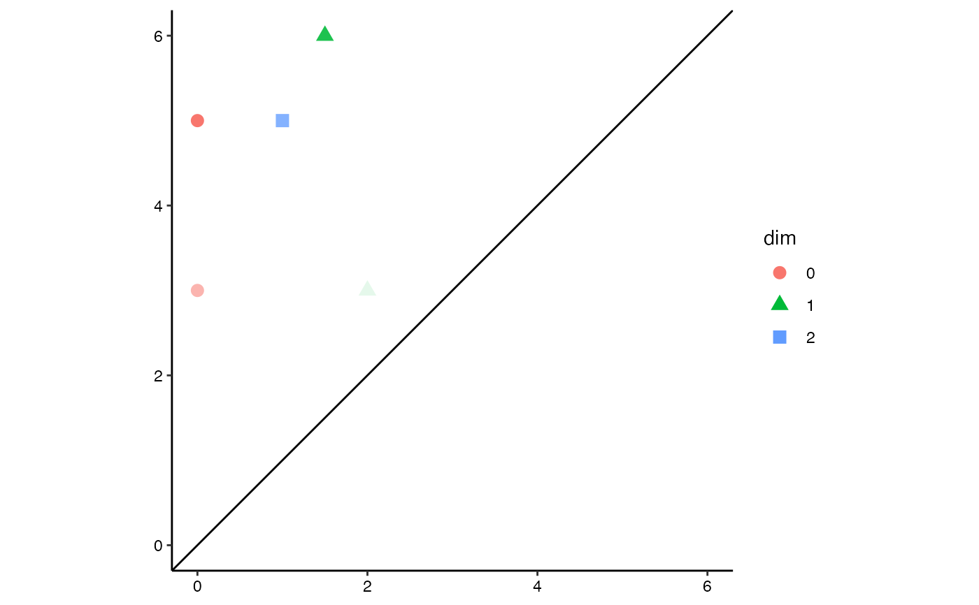
Persistence diagrams are scatterplots of persistence data.

Persistence data

Persistence data encode the values of an underlying parameter \(\epsilon\) at which topological features appear ("birth") and disappear ("death"). The difference between the birth and the death of a feature is called its persistence. Whereas topological features may be of different dimensions, persistence data sets usually also include the dimension of each feature.

ggtda expects persistence data to have at least three columns: birth, death, and dimension.

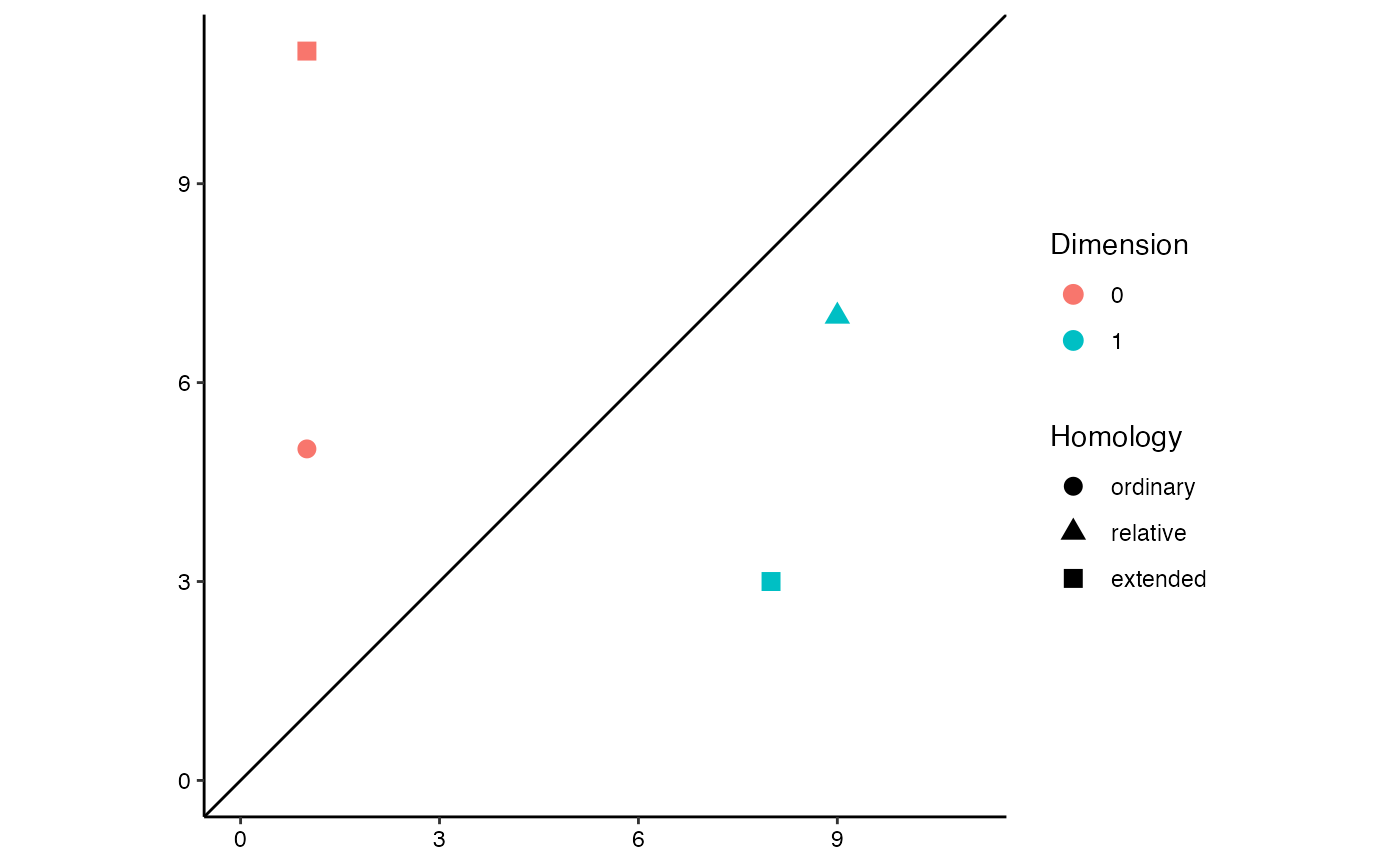
Persistence diagrams recognize extended persistence data, with negative birth/death values arising from the relative part of the filtration.

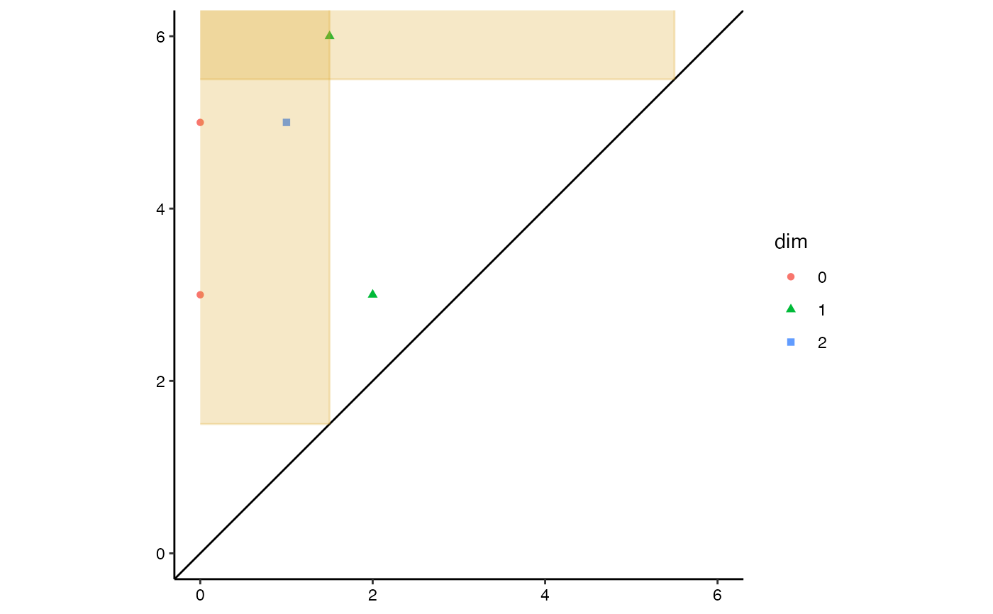
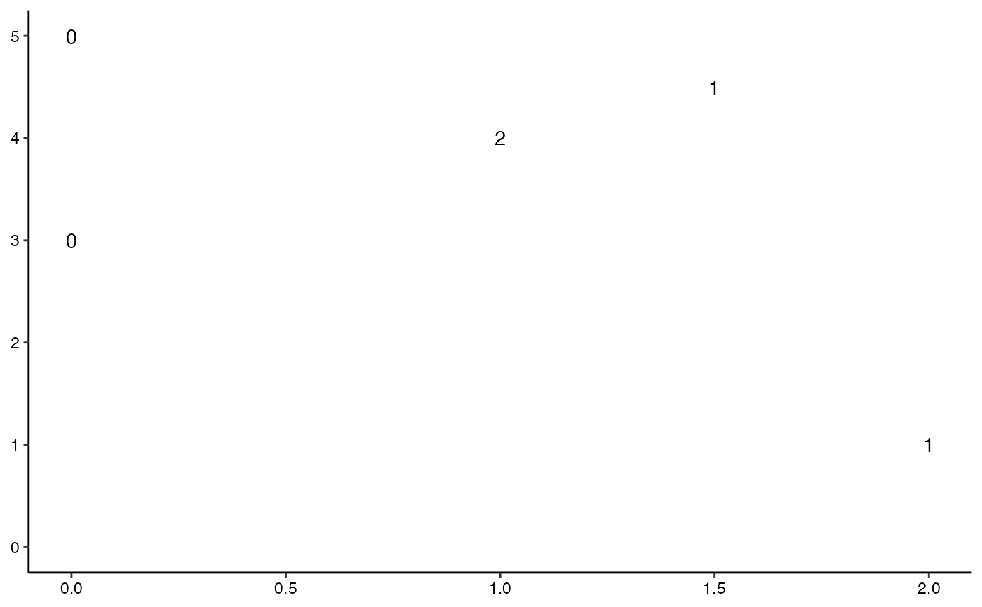
The original persistence diagrams plotted persistence against birth in what we call "flat" diagrams, but most plot death against birth in "diagonal" diagrams, often with a diagonal line indicating zero persistence.

The geom_fundamental_box() layer renders fundamental boxes at specified time points (Chung & Lawson, 2020).

Aesthetics

stat_persistence() understands the following aesthetics (required aesthetics are in bold):

start or dataset
end or dataset
group

geom_fundamental_box() understands the following aesthetics (required aesthetics are in bold):

alpha
colour
fill
group
linetype
linewidth

Learn more about setting these aesthetics in vignette("ggplot2-specs", package = "ggplot2").

Computed variables

stat_persistence calculates the following variables that can be accessed with delayed evaluation.

after_stat(start)
birth value of each feature (from 'dataset' aesthetic).
after_stat(end)
death value of each feature (from 'dataset' aesthetic).
after_stat(dimension)
integer feature dimension (from 'dataset' aesthetic).
after_stat(group)
interaction of existing 'group', dataset ID, and 'dimension'.
after_stat(id)
character feature identifier (across 'group').
after_stat(part)
whether features belong to ordinary, relative, or extended homology.
after_stat(persistence)
differences between birth and death values of features.

References

H Edelsbrunner, D Letscher, and A Zomorodian (2000) Topological persistence and simplification. Proceedings 41st Annual Symposium on Foundations of Computer Science, 454--463. doi:10.1109/SFCS.2000.892133

H Edelsbrunner and D Morozov (2012) Persistent Homology: Theory and Practice. European Congress of Mathematics, 31--50. doi:10.4171/120

Y-M Chung and A Lawson (2020) Persistence Curves: A Canonical Framework for Summarizing Persistence Diagrams. https://arxiv.org/abs/1904.07768

Examples


# toy example
toy.data <- data.frame(
  birth = c(0, 0, 1, 2, 1.5),
  death = c(5, 3, 5, 3, 6),
  dim = c("0", "0", "2", "1", "1")
)
# diagonal persistence diagram, coding persistence to transparency
ggplot(toy.data,
       aes(start = birth, end = death, colour = dim, shape = dim)) +
  theme_persist() +
  coord_equal() +
  stat_persistence(aes(alpha = after_stat(persistence)),
                   diagram = "diagonal", size = 3) +
  geom_abline(intercept = 0, slope = 1) +
  lims(x = c(0, 6), y = c(0, 6)) +
  guides(alpha = "none")

# diagonal persistence diagram with fundamental boxes
ggplot(toy.data,
       aes(start = birth, end = death, colour = dim, shape = dim)) +
  theme_persist() +
  coord_equal() +
  stat_persistence() +
  geom_abline(intercept = 0, slope = 1) +
  geom_fundamental_box(t = c(1.5, 5.5),
                       color = "goldenrod", fill = "goldenrod") +
  lims(x = c(0, 6), y = c(0, 6)) +
  guides(alpha = "none")

# flat persistence diagram, coding dimension to numeral
ggplot(toy.data,
       aes(start = birth, end = death, label = dim)) +
  theme_persist() +
  stat_persistence(diagram = "flat", geom = "text") +
  lims(x = c(0, NA), y = c(0, NA))

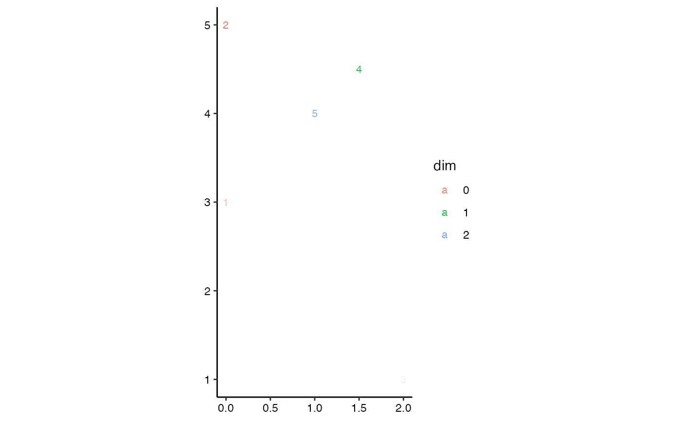
# flat persistence diagram, labeling by feature ID
ggplot(toy.data, aes(start = birth, end = death, colour = dim, shape = dim)) +
  theme_persist() +
  coord_equal() +
  stat_persistence(
    geom = "text",
    aes(label = after_stat(id), alpha = after_stat(persistence)),
    diagram = "flat", size = 3
  ) +
  guides(alpha = "none")


# toy extended persistence data, adapted from Carriere & Oudot (2015)
eph.data <- data.frame(
  dimension = c(0L, 1L, 0L, 1L),
  birth = c(1, -9, 1, 8),
  death = c(5, -7, -11, -3)
)
# extended persistence diagram
ggplot(eph.data,
       aes(start = birth, end = death, color = factor(dimension))) +
  theme_persist() +
  coord_equal() +
  stat_persistence(aes(shape = after_stat(part)), size = 3) +
  geom_abline(intercept = 0, slope = 1) +
  lims(x = c(0, 11), y = c(0, 11)) +
  labs(color = "Dimension", shape = "Homology")

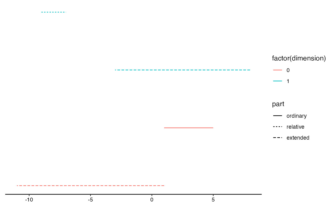
# extended barcode
ggplot(eph.data,
       aes(start = birth, end = death, color = factor(dimension))) +
  theme_barcode() +
  geom_barcode(aes(linetype = after_stat(part)))


# list-column of data sets to 'dataset' aesthetic
raw_data <- data.frame(obj = I(list(eurodist, 10*swiss, Nile)))
raw_data$class <- vapply(raw_data$obj, class, "")

if ("TDA" %in% rownames(utils::installed.packages())) {
  
  # barcodes
  ggplot(raw_data, aes(dataset = obj)) +
    geom_barcode(aes(color = factor(after_stat(dimension))),
                 engine = "TDA") +
    facet_wrap(facets = vars(class))
  # persistence diagram
  ggplot(raw_data, aes(dataset = obj)) +
    stat_persistence(aes(color = factor(after_stat(dimension)), shape = class),
                     engine = "GUDHI")
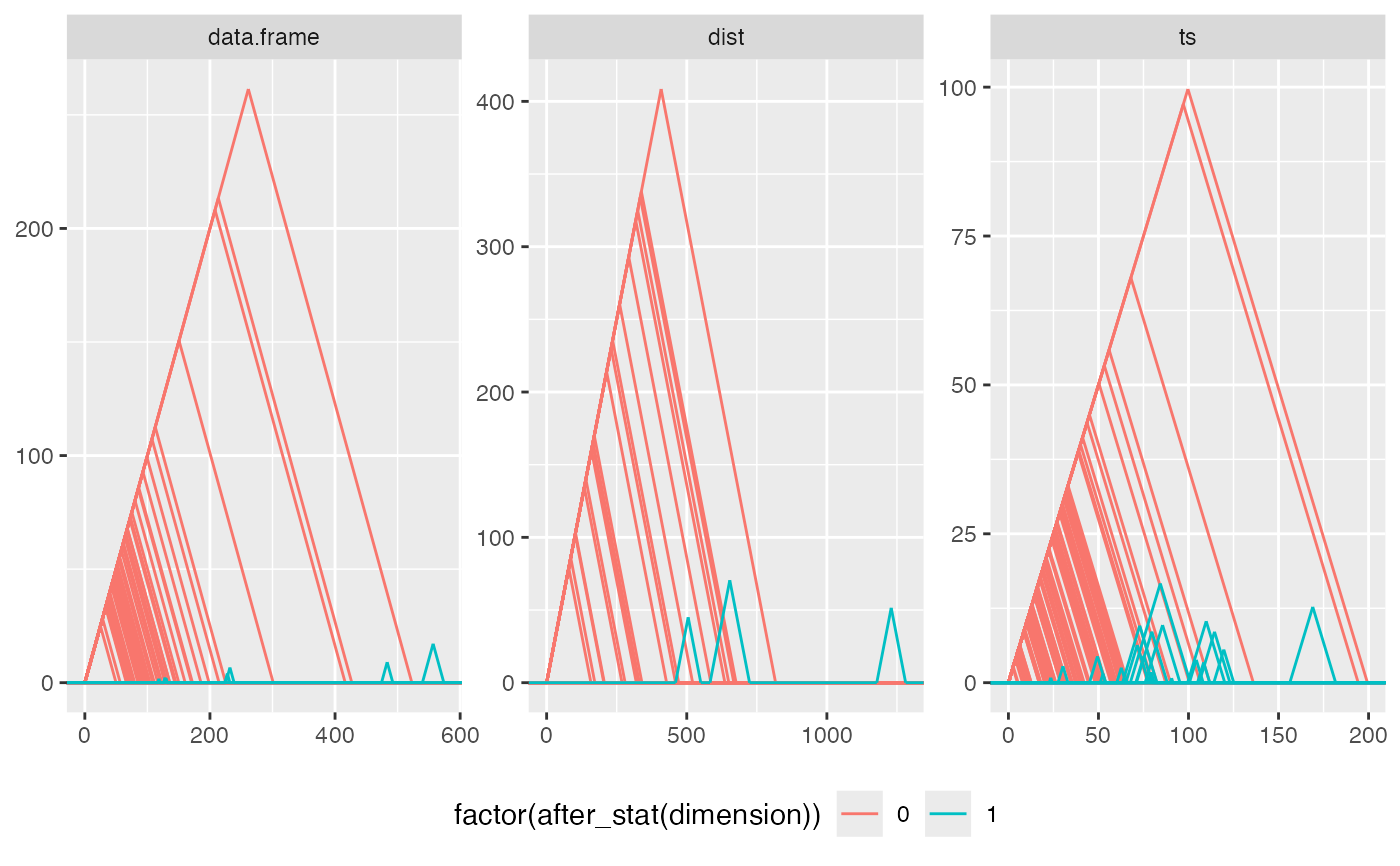
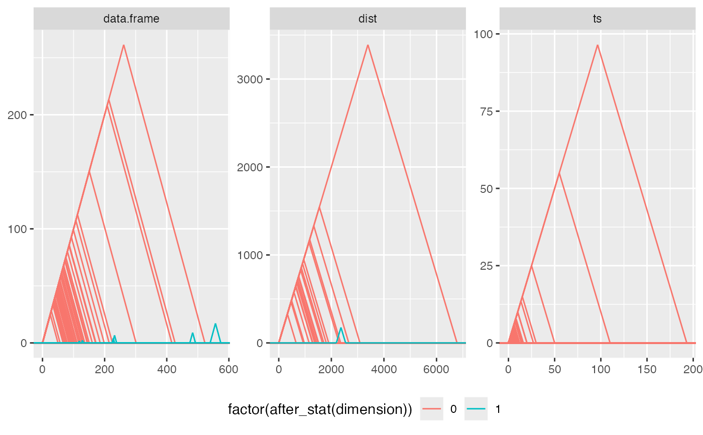
  # persistence landscape
  ggplot(raw_data, aes(dataset = obj)) +
    facet_wrap(facets = vars(class), scales = "free") +
    stat_landscape(aes(color = factor(after_stat(dimension))),
                   engine = "Dionysus") +
    theme(legend.position = "bottom")
  
}
#> Warning: Removed 3 rows containing non-finite outside the scale range
#> (`stat_landscape()`).


if ("ripserr" %in% rownames(utils::installed.packages())) {
  
  # exclude time series data if {ripserr} v0.1.1 is installed
  if (utils::packageVersion("ripserr") == "0.1.1")
    raw_data <- raw_data[c(1L, 2L), ]
  # barcodes
  ggplot(raw_data, aes(dataset = obj)) +
    geom_barcode(aes(color = factor(after_stat(dimension))),
                 engine = "ripserr") +
    facet_wrap(facets = vars(class))
  # persistence diagram
  ggplot(raw_data, aes(dataset = obj)) +
    stat_persistence(aes(color = factor(after_stat(dimension)), shape = class),
                     engine = "ripserr")
  # persistence landscape
  ggplot(raw_data, aes(dataset = obj)) +
    facet_wrap(facets = vars(class), scales = "free") +
    stat_landscape(aes(color = factor(after_stat(dimension))),
                   engine = "ripserr") +
    theme(legend.position = "bottom")
  
}

Persistence diagrams

Arguments

Details

Persistence data