Persistence landscapes

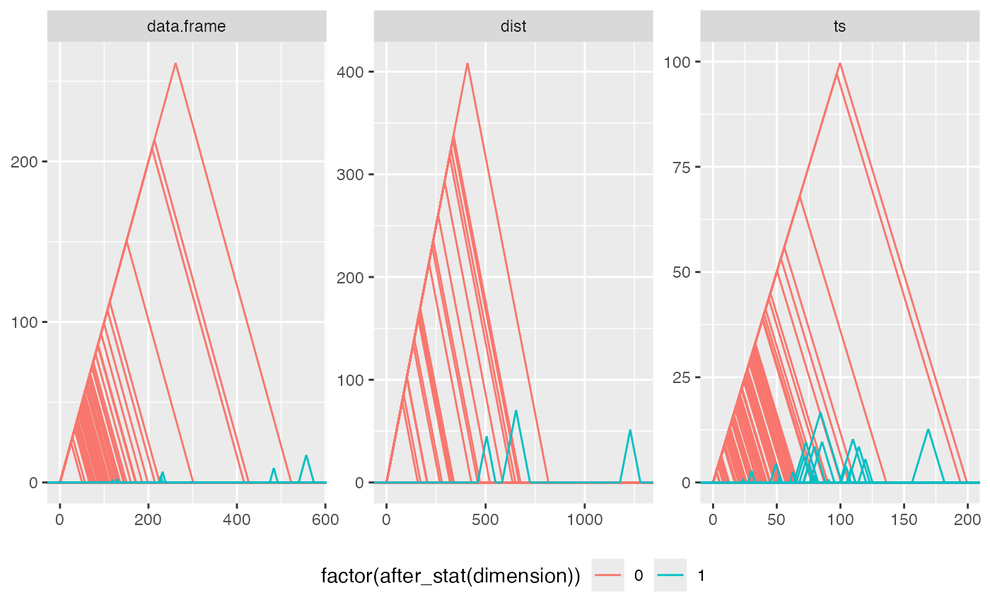
Visualize persistence data as a persistence landscape.

stat_landscape(
  mapping = NULL,
  data = NULL,
  geom = "landscape",
  position = "identity",
  filtration = "Rips",
  diameter_max = NULL,
  radius_max = NULL,
  dimension_max = 1L,
  field_order = 2L,
  engine = NULL,
  diagram = "landscape",
  n_levels = Inf,
  na.rm = FALSE,
  show.legend = NA,
  inherit.aes = TRUE,
  ...
)

geom_landscape(
  mapping = NULL,
  data = NULL,
  stat = "landscape",
  position = "identity",
  lineend = "butt",
  linejoin = "round",
  linemitre = 10,
  na.rm = FALSE,
  show.legend = NA,
  inherit.aes = TRUE,
  ...
)

Arguments

mapping

Set of aesthetic mappings created by aes(). If specified and inherit.aes = TRUE (the default), it is combined with the default mapping at the top level of the plot. You must supply mapping if there is no plot mapping.

data

The data to be displayed in this layer. There are three options:

If NULL, the default, the data is inherited from the plot data as specified in the call to ggplot().

A data.frame, or other object, will override the plot data. All objects will be fortified to produce a data frame. See fortify() for which variables will be created.

A function will be called with a single argument, the plot data. The return value must be a data.frame, and will be used as the layer data. A function can be created from a formula (e.g. ~ head(.x, 10)).

geom

The geometric object to use to display the data, either as a ggproto Geom subclass or as a string naming the geom stripped of the geom_ prefix (e.g. "point" rather than "geom_point")

position

Position adjustment, either as a string naming the adjustment (e.g. "jitter" to use position_jitter), or the result of a call to a position adjustment function. Use the latter if you need to change the settings of the adjustment.

filtration

The type of filtration from which to compute persistent homology; one of "Rips", "Vietoris" (equivalent) or "alpha".

diameter_max, radius_max

Maximum diameter or radius for the simplicial filtration. Both default to NULL, in which case the complete filtration is constructed.

dimension_max

Maximum dimension of the simplicial filtration.

field_order

(Prime) order of the field over which to compute persistent homology.

engine

The computational engine to use (see 'Details'). Reasonable defaults are chosen based on filtration.

diagram

One of "flat", "diagonal", or "landscape"; the orientation for the diagram should take.

n_levels

The number of levels to compute and plot. If Inf (the default), determined to be all levels.

na.rm

If FALSE, the default, missing values are removed with a warning. If TRUE, missing values are silently removed.

show.legend

logical. Should this layer be included in the legends? NA, the default, includes if any aesthetics are mapped. FALSE never includes, and TRUE always includes. It can also be a named logical vector to finely select the aesthetics to display.

inherit.aes

If FALSE, overrides the default aesthetics, rather than combining with them. This is most useful for helper functions that define both data and aesthetics and shouldn't inherit behaviour from the default plot specification, e.g. borders().

...

Other arguments passed on to layer(). These are often aesthetics, used to set an aesthetic to a fixed value, like colour = "red" or size = 3. They may also be parameters to the paired geom/stat.

stat

The statistical transformation to use on the data for this layer, either as a ggproto Geom subclass or as a string naming the stat stripped of the stat_ prefix (e.g. "count" rather than "stat_count")

lineend

Line end style (round, butt, square).

linejoin

Line join style (round, mitre, bevel).

linemitre

Line mitre limit (number greater than 1).

Details

Persistence landscapes, anticipated by some alternative coordinatizations of persistence diagrams, were proposed as Lipschitz functions that demarcate the Pareto frontiers of persistence diagrams. They can be averaged over the diagrams obtained from multiple data sets designed or hypothesized to have been generated from the same underlying topological structure.

Persistence landscapes do not currently recognize extended persistence data.

Aesthetics

stat_landscape() understands the following aesthetics (required aesthetics are in bold):

start or dataset
end or dataset
group

geom_landscape() understands the following aesthetics (required aesthetics are in bold):

x
y
alpha
colour
group
linetype
linewidth

Learn more about setting these aesthetics in vignette("ggplot2-specs", package = "ggplot2").

Computed variables

stat_landscape calculates the following variables that can be accessed with delayed evaluation.

after_stat(x), after_stat(y)
coordinates of segment endpoints of each frontier.
after_stat(dimension)
feature dimension (with 'dataset' aesthetic only).
after_stat(group)
interaction of existing 'group', dataset ID, and 'dimension'.
after_stat(level)
position of each frontier, starting from the outermost.
after_stat(slope)
slope of the landscape abscissa.

Note that start and end are dropped during the statistical transformation.

References

P Bubenik (2015) Statistical Topological Data Analysis using Persistence Landscapes. Journal of Machine Learning Research, 16 77--102. http://jmlr.org/papers/v16/bubenik15a.html

F Chazal and B Michel (2017) An introduction to Topological Data Analysis: fundamental and practical aspects for data scientists. https://arxiv.org/abs/1710.04019

Examples

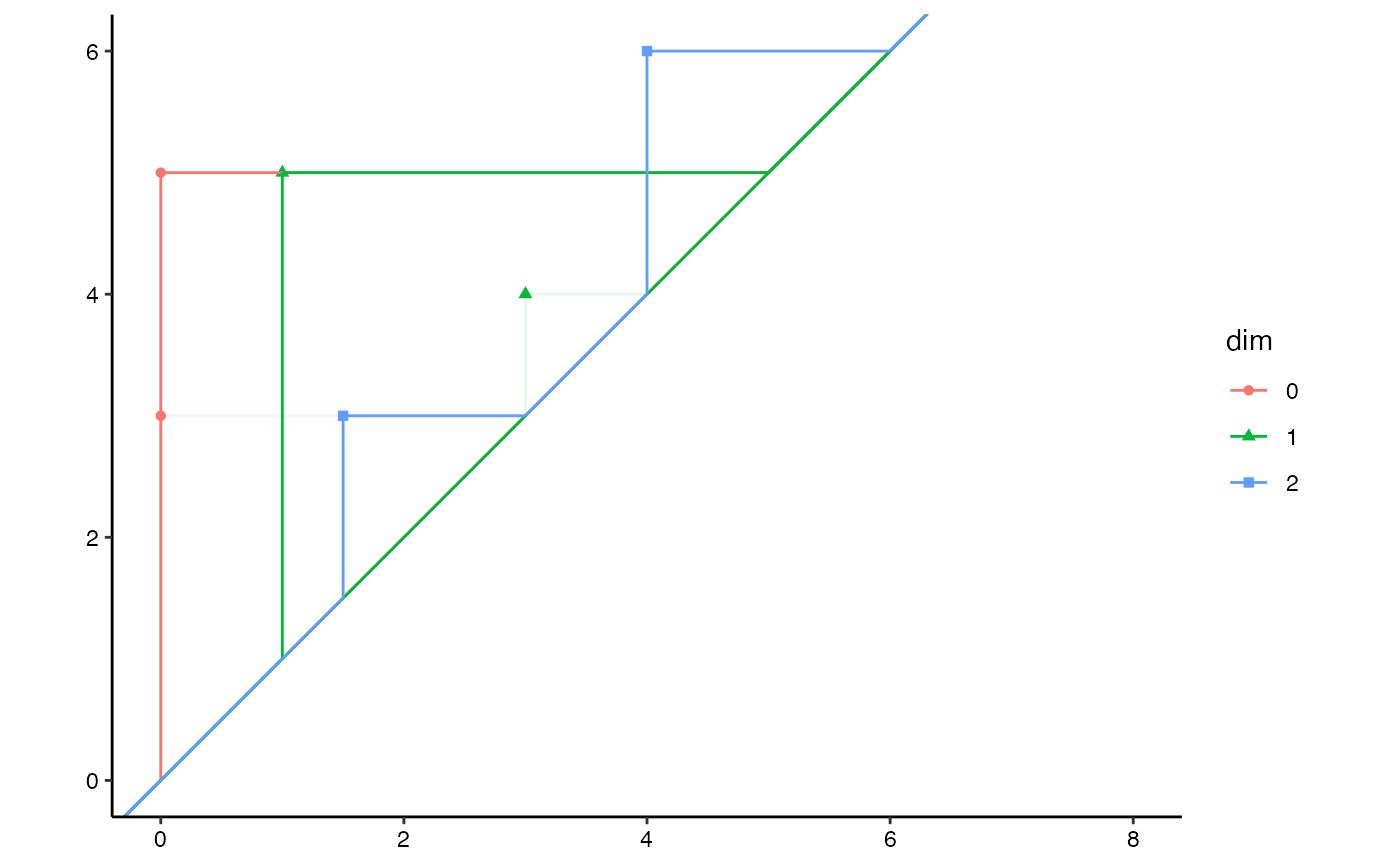
# toy example
toy.data <- data.frame(
  birth = c(0, 0, 1, 3, 4, 1.5),
  death = c(5, 3, 5, 4, 6, 3),
  dim = factor(c(0, 0, 1, 1, 2, 2))
)
# persistence diagram with landscape overlaid
ggplot(toy.data,
       aes(start = birth, end = death, colour = dim, shape = dim)) +
  theme_persist() +
  coord_equal() +
  stat_persistence() +
  stat_landscape(aes(alpha = -after_stat(level)), diagram = "diagonal") +
  lims(x = c(0, 8), y = c(0, NA)) +
  guides(alpha = "none")

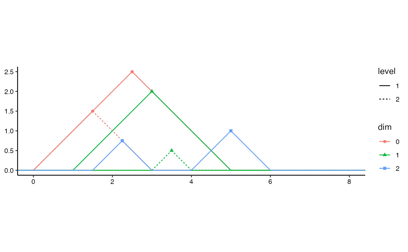
# persistence landscape with diagram overlaid
ggplot(toy.data,
       aes(start = birth, end = death, colour = dim, shape = dim)) +
  theme_persist() +
  coord_equal() +
  stat_landscape(aes(linetype = after_stat(factor(level)))) +
  stat_persistence(diagram = "landscape") +
  lims(x = c(0, 8), y = c(0, NA)) +
  labs(linetype = "level")


# load library and generate dataset for comprehensive example
library("ripserr")
# noisy unit circle (Betti-1 number = 1)
n <- 100L; sd <- 0.1
set.seed(7)
t <- stats::runif(n = n, min = 0, max = 2*pi)
annulus.df <- data.frame(
  x = cos(t) + stats::rnorm(n = n, mean = 0, sd = sd),
  y = sin(t) + stats::rnorm(n = n, mean = 0, sd = sd)
)
# calculate persistence homology and format
annulus.phom <- as.data.frame(vietoris_rips(annulus.df))
annulus.phom$dimension <- as.factor(annulus.phom$dimension)
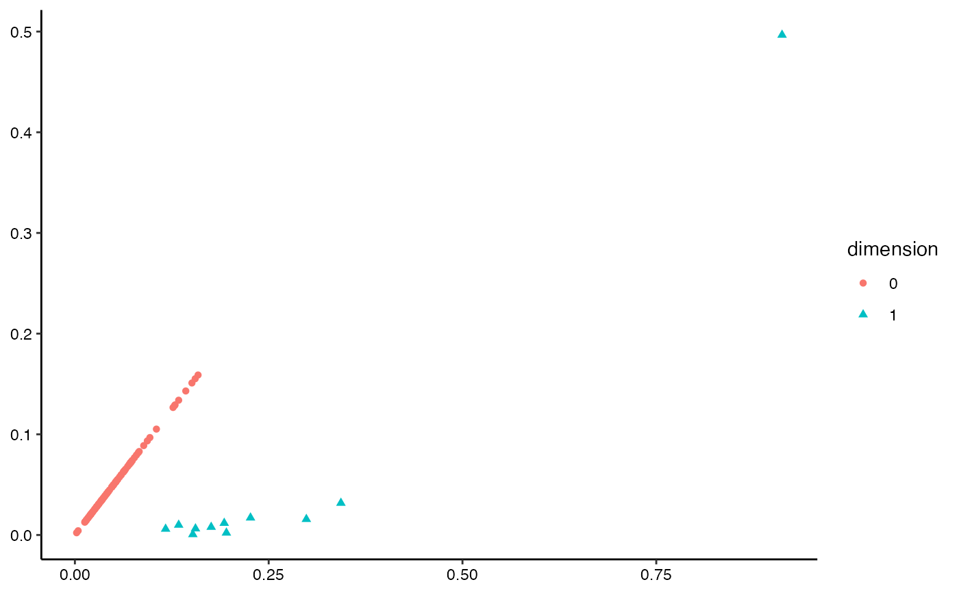
# pretty diagonal persistence diagram
ggplot(annulus.phom, aes(start = birth, end = death,
                         shape = dimension, colour = dimension)) +
  stat_persistence(diagram = "landscape") +
  theme_persist()

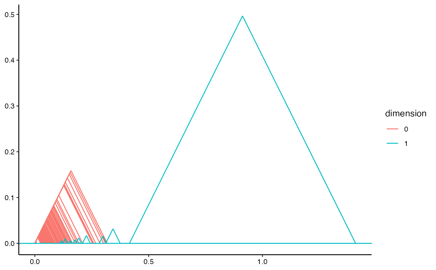
# pretty landscape persistence diagram
ggplot(annulus.phom, aes(start = birth, end = death,
                         shape = dimension, colour = dimension)) +
  stat_landscape(diagram = "landscape") +
  theme_persist()


# list-column of data sets to 'dataset' aesthetic
raw_data <- data.frame(obj = I(list(eurodist, 10*swiss, Nile)))
raw_data$class <- vapply(raw_data$obj, class, "")

if ("TDA" %in% rownames(utils::installed.packages())) {
  
  # barcodes
  ggplot(raw_data, aes(dataset = obj)) +
    geom_barcode(aes(color = factor(after_stat(dimension))),
                 engine = "TDA") +
    facet_wrap(facets = vars(class))
  # persistence diagram
  ggplot(raw_data, aes(dataset = obj)) +
    stat_persistence(aes(color = factor(after_stat(dimension)), shape = class),
                     engine = "GUDHI")
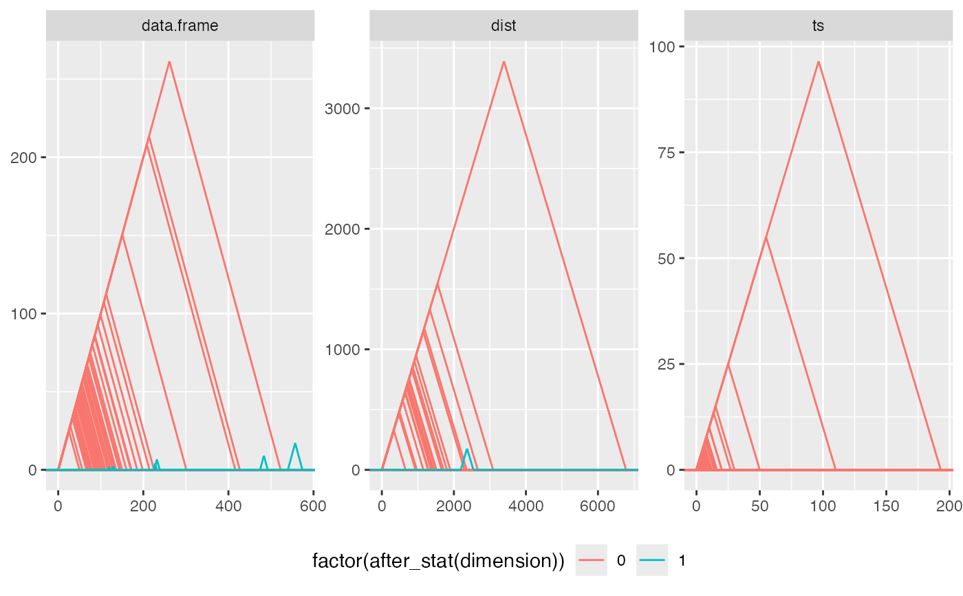
  # persistence landscape
  ggplot(raw_data, aes(dataset = obj)) +
    facet_wrap(facets = vars(class), scales = "free") +
    stat_landscape(aes(color = factor(after_stat(dimension))),
                   engine = "Dionysus") +
    theme(legend.position = "bottom")
  
}
#> Warning: Removed 3 rows containing non-finite outside the scale range
#> (`stat_landscape()`).


if ("ripserr" %in% rownames(utils::installed.packages())) {
  
  # exclude time series data if {ripserr} v0.1.1 is installed
  if (utils::packageVersion("ripserr") == "0.1.1")
    raw_data <- raw_data[c(1L, 2L), ]
  # barcodes
  ggplot(raw_data, aes(dataset = obj)) +
    geom_barcode(aes(color = factor(after_stat(dimension))),
                 engine = "ripserr") +
    facet_wrap(facets = vars(class))
  # persistence diagram
  ggplot(raw_data, aes(dataset = obj)) +
    stat_persistence(aes(color = factor(after_stat(dimension)), shape = class),
                     engine = "ripserr")
  # persistence landscape
  ggplot(raw_data, aes(dataset = obj)) +
    facet_wrap(facets = vars(class), scales = "free") +
    stat_landscape(aes(color = factor(after_stat(dimension))),
                   engine = "ripserr") +
    theme(legend.position = "bottom")
  
}