Two-sample test for functional representations of persistence homology data

This function performs a two-sample test for persistence homology data using the theory of permutation hypothesis testing to test the null hypothesis that the two samples come from the same distribution. The input data must be objects of class persistence_set typically produced by phutil::as_persistence_set().

Usage

two_sample_functional_test(
  x,
  y,
  dimension = 0L,
  scale_size = 100L,
  representation = c("betti", "euler", "life", "silhouette", "entropy"),
  mu = 0,
  order = 2L,
  nknots = scale_size,
  B = 1000L,
  paired = FALSE
)

Arguments

x: An object of class persistence_set typically produced by phutil::as_persistence_set() specifying the first sample.
y: An object of class persistence_set typically produced by phutil::as_persistence_set() specifying the second sample.
dimension: An integer value specifying the homology dimension to use. Defaults to 0L, which corresponds to the 0-dimensional homology.
scale_size: An integer value specifying the number of scale values to use for the functional representation. Defaults to 100L.
representation: A string specifying the functional representation to use. Choices are "betti", "euler", "life", "silhouette", and "entropy". Defaults to "betti".
mu: The difference between the first functional population and the second functional population under the null hypothesis. Either a constant (in this case, a constant function is used) or a J-dimensional vector containing the evaluations on the same grid which data are evaluated. The default is mu=0.
order: Order of the B-spline basis expansion. The default is order=2.
nknots: An integer value specifying the number of knots to use for the B-spline representation. Defaults to scale_size.
B: An integer value specifying the number of permutations to use for the permutation hypothesis test. Defaults to 1000L.
paired: A logical indicating whether the test is paired. The default is FALSE.

Value

A length-4 list containing the following objects:

xfd: A numeric matrix of shape \(n_1 \times p\) storing the representation of the first sample on a uniform grid.
yfd: A numeric matrix of shape \(n_2 \times p\) storing the representation of the second sample on a uniform grid.
scale_seq: A numeric vector of shape \(p\) storing the scale sequence used for the functional representation.
iwt: An object of class ITP2 which is a list containing at least the following components:
- basis: A string indicating the basis used for the first phase of the algorithm. In this case, equals to "B-spline".
- test: A string indicating the type of test performed. In this case, equals to "2pop".
- mu: The difference between the mean of the first and second populations under the null hypothesis (as entered by the user).
- paired: A boolean value indicating whether the two samples are paired or not (as entered by the user).
- coeff: A numeric matrix of shape \(n \times p\) of the \(p\) coefficients of the B-spline basis expansion, with \(n = n_1 + n_2\). Rows are associated to units and columns to the basis index. The first \(n_1\) rows report the coefficients of the first population units and the following \(n_2\) rows report the coefficients of the second population units.
- pval: A numeric vector of shape \(p\) storing the uncorrected p-values for each coefficient of the B-spline basis expansion.
- pval.matrix: A numeric matrix of shape \(p \times p\) of the p-values of the multivariate tests. The element \((i, j)\) of the pval.matrix matrix contains the p-value of the joint NPC test of the components \((j, j+1, \dots, j+(p-i))\).
- corrected.pval: A numeric vector of shape \(p\) storing the corrected p-values for each coefficient of the B-spline basis expansion.
- labels: A character vector of shape \(n\) storing the membership of each unit to the first or second population.
- data.eval: A numeric matrix of shape \(n \times p\) storing the evaluation of the functional data on a uniform grid.
- heatmap.matrix: A numeric matrix storing the p-values. Used only for plots.

References

Pini, A., & Vantini, S. (2017). Interval-wise testing for functional data. Journal of Nonparametric Statistics, 29(2), 407-424.

Examples

tref1 <- trefoils1[1:5]
archsp <- archspirals[1:5]
out <- two_sample_functional_test(tref1, archsp, B = 10L, scale_size = 20L)
#> [1] "First step: basis expansion"
#> Swapping 'y' and 'argvals', because 'y' is  simpler,
#>   and 'argvals' should be;  now  dim(argvals) =  19 ;  dim(y) =  19 x 10 
#> [1] "Second step: joint univariate tests"
#> [1] "Third step: interval-wise combination and correction"
#> [1] "creating the p-value matrix: end of row 2 out of 19"
#> [1] "creating the p-value matrix: end of row 3 out of 19"
#> [1] "creating the p-value matrix: end of row 4 out of 19"
#> [1] "creating the p-value matrix: end of row 5 out of 19"
#> [1] "creating the p-value matrix: end of row 6 out of 19"
#> [1] "creating the p-value matrix: end of row 7 out of 19"
#> [1] "creating the p-value matrix: end of row 8 out of 19"
#> [1] "creating the p-value matrix: end of row 9 out of 19"
#> [1] "creating the p-value matrix: end of row 10 out of 19"
#> [1] "creating the p-value matrix: end of row 11 out of 19"
#> [1] "creating the p-value matrix: end of row 12 out of 19"
#> [1] "creating the p-value matrix: end of row 13 out of 19"
#> [1] "creating the p-value matrix: end of row 14 out of 19"
#> [1] "creating the p-value matrix: end of row 15 out of 19"
#> [1] "creating the p-value matrix: end of row 16 out of 19"
#> [1] "creating the p-value matrix: end of row 17 out of 19"
#> [1] "creating the p-value matrix: end of row 18 out of 19"
#> [1] "creating the p-value matrix: end of row 19 out of 19"
#> [1] "Interval Testing Procedure completed"
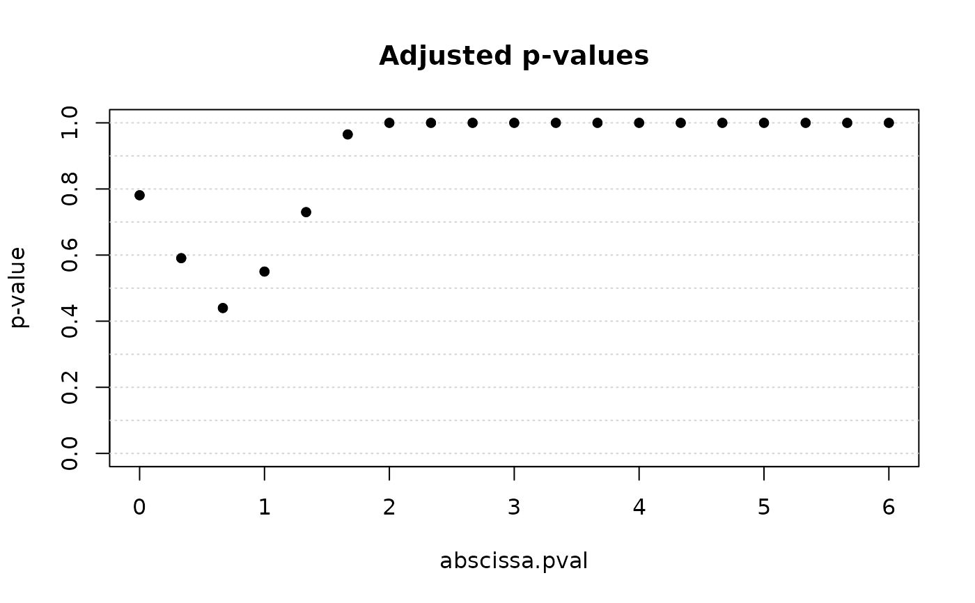
plot(out$iwt, xrange = range(out$scale_seq))


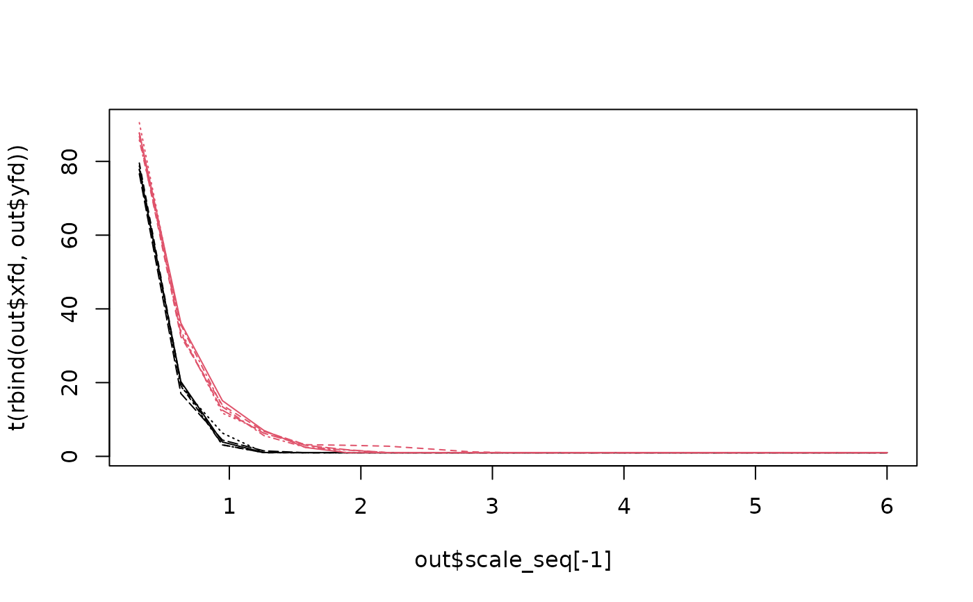
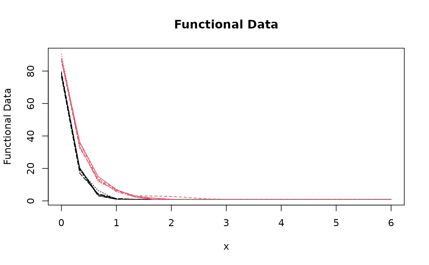
matplot(
  out$scale_seq[-1],
  t(rbind(out$xfd, out$yfd)),
  type = "l",
  col = c(rep(1, length(tref1)), rep(2, length(archsp)))
)